Nature Photography

Noise reduction is one of the most fundamental aspects of astrophotography processing. We work with images of minimal signal to noise ratio, a ratio that for best results must be increased, often by a significant amount, in order to produce a quality image. Ironically, given it’s importance, noise reduction is one of the most misunderstood, and possibly one of the least understood, aspects of image processing. PixInsight provides a wide range of powerful noise reduction tools that can assist us in the pursuit of lower noise and higher SNR. These tools are often so powerful, however, that the inevitable result, if you are not already familiar with them (and possibly even if you are) is artifact-ridden, plasticized images that have a very artificial look and feel.

LINEAR PHASE

As with most processing in PixInsight, the first phase of noise reduction will take place on linear (unstretched) data. Personally, I try to perform as much processing as I can on the linear data, as once you start stretching, the consistency of the data is lost, and along with it goes the consistency of your workflow. There are several benefits to processing linear data. Outside of the consistency of the data, it is usually more deterministic (especially if you have performed a linear fit before any other processing). Noise can also be better modeled when the data is linear, and this can be important for some noise reduction tools.

It should be noted that noise reduction is best performed on images where any gradients have already been extracted, and where proper color calibration has already been performed. The reasons for this are two fold. First, removal of gradients often reveals the true nature of the noise remaining within the object image, as gradients often increase (sometimes significantly) the signal strength. Removal of that extra signal will offset the signal, but leave behind it’s noise, as noise cannot be subtracted or offset…only reduced. Second, color calibration will often shift color channels around. Particularly with DSLR data (especially unmodded or LP filtered data), certain color channels may have significantly more or less signal strength than others, resulting in large discrepancies in noise levels. Color calibration will realign each channel, and that can often result in increases in noise in one channel or another. It is important that these changes take place BEFORE noise reduction. That allows any noise reduction to more effectively target the remnant noise overall.

With linear phase noise reduction, our primary goals are:

• Banding removal
• Primary chromatic noise reduction
• High frequency noise reduction
• Medium and low frequency noise reduction
  • Luminance & Chrominance

These goals may require multiple passes with a given NR tool. Banding is listed as it should really be the first thing we tackle, before any other processing has been done. This actually includes any gradient removal or color correction, as the nature of banding reduction is different than most other noise reduction. This is performed with the CanonBandingReduction (CBR) script, which can be found under Script -> Utilities -> CanonBandingReduction. This tool only performs horizontal banding reduction natively, which means to correct vertical banding, which is often more common, you must first rotate the image data by 90 degrees. This rotation can be done with the FastRotation tool by simply choosing Rotate 90° Counter-clockwise and applying to the image before running the CBR script. Re-apply FastRotation by choosing Rotate 90° Clockwise after you have finished with CBR.

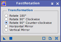The CBR script is a less than ideally implemented script. It really needs some debouncing delays so that you can adjust sliders without issue, however as it is currently written, if you have the preview enabled (which is usually necessary with linear data), the script will re-render every tick of adjustment made by a slider. This can result in the tool being rather frustrating to use. The solution to this is to disable the preview before making any adjustments, then manually re-enable it. Tedious, but it does speed up the use of the tool. You should adjust the amount up and down to see what effect it has. If your going the wrong way, your banding will actually increase rather than decrease. An amount less than 1.0 is often necessary with fainter banding. You may find that you need to run this script a couple of times to fully eliminate the banding in your image, however be careful with more than one pass. This script can affect detail.

Primary Chromatic Noise Reduction

After banding reduction (if it was necessary) and after color calibration, we want to correct any primary color cast in the data. What kind of color cast you may have will often depend on the nature of your data, both the kind of camera used (mono CCD or CFA DSLR) as well as the kind of filters used, channel offsets, and relative SNRs across each channel. With CCD data it often depends on the filters used and how much integration time you acquired for each, and if there are SNR discrepancies, that will usually show up as a stronger color in chrominance noise. With DSLR data, it usually depends on whether the camera is astro modded or not and what kind of LP filter you used, if any. In the case of both, the amount of light pollution present can also play a role in channel shift and relative SNR.

Regardless of the specifics, SCNR is the proper tool to use to correct the primary color cast that results from such channel and SNR discrepancies. SCNR or Subtractive Chromatic Noise Reduction, aims to normalize the standard distribution of noise across the channels by adjusting one of them. In most cases, the primary color cast present in any image will be a green one. This is in part due to the fact that green is not a color most nebula emit, although stars do emit green, and perceptually we recognize fairly easily when there is too much green. Additionally, in the case of DSLR data, there are usually twice as many green pixels as red or blue pixels, which definitely changes the standard deviation of noise in that channel, and usually results in a discrepancy in SNR. Regardless of the cause, applying SCNR to the image will correct the cast.

SCNR Histogram: Before (Left) & After (Right); Note subtractive shift in green channel and normalization with other channels.

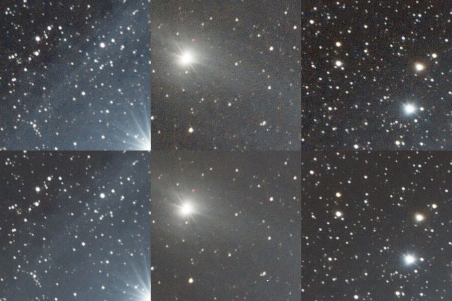
I won’t go into detail about how to use SCNR to it’s fullest here. In the simplest of terms, I apply SCNR, usually to the green channel, although sometimes to the red channel if the dominant cast is reddish, with a Protection Method of Average Neutral. I will usually apply it with an amount between 0.5 and 0.8, enabling the Preserve Lightness option. This removes the primary color cast, without overly decimating the corrected color channel. Too much reduction (many often run SCNR at 1.0) and you will often realize a visible loss in star color diversity. If you have properly applied SCNR, you should observe a correction similar to the following:

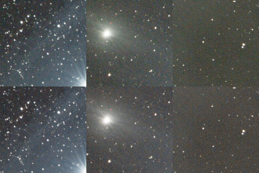
SCNR Befor and After Comparison; (Note that I did not clean this data with CosmeticCorrection, and note the effect the hot pixel has in the middle panel)

High Frequency Noise Reduction

TGVDenoise Dialog

The first kind of general noise we want to tackle in our images is high frequency noise. I often call this per-pixel noise, as that is effectively the highest frequency noise we can see in our images. High frequency noise is a primary type of noise, the primary form that random noise takes, and is contributed to by read noise, dark current, skyfog shot noise as well as the shot noise in the object image itself. There are two tools that can handle high frequency noise that I use most often: TGVDenoise (TGV) , and MultiscaleMedianTransform (MMT) . For the first pass of high frequency noise reduction, my tool of choice is a properly attenuated TGV, rather than MMT. I find the nature of MMT makes it more suited to medium and lower frequency noise correction, and a second pass of high frequency noise correction.

TGV has a lot of options, however in this particular context I am not going to go into each of them in detail. I will cover the tool in more detail in the PixInsights article dedicated to it. For now, I am going to cover my general usage pattern for most of the images I process.

TGV can be applied in two primary modes, RGB/K and CIE L*a*b*. I generally prefer the Lab mode, as it allows me to configure lightness noise correction separately from chrominance. Note here the use of the term Lightness. In PixInsight, there are two types of luminance channels. Lightness and Luminance. The former, in the context of PixInsight, is always used to refer to the L* channel of L*a*b* data. The latter is always used to the Y channel of Y/cb/cr data. These two types of luminance extractions differ algorithmically, and there are nuanced changes to the data, but generally speaking, they both referr to the colorless grayscale representation of pixel intensities. Conversely, Chrominance referrs to either the a*b* or cb/cr channels, depending on which algorithm is used.

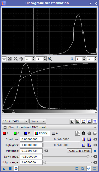
Before doing anything with TGV, it is important that we generate a proper mask to attenuate the effect and preserve both fine detail as well as the fine grained nature of high frequency noise. Preservation of both detail and grain is one of the key tenets of my approach, and proper masking achieves both. Fine grain is critical to avoid plasticization of you images, and it is generally more aesthetically pleasing than ultra smooth truly noiseless data.

Generating a mask for TGV is pretty strait forward. Start by extracting a luminance channel from your image. The simplest way to do this is by clicking the Extract CIE L* component button on the toolbar. Once you have the luminance channel, apply a standard STF to it, then apply that STF to the image via HistogramTransformation (HT). This will stretch the mask, which is essential for it to function properly, as a value of 1.0 means 100% protection and a value of 0.0 means 0% protection. Rename this mask, adding “_Lum_mask” to the end of the original name for the image (remove any _clone part of the name). Duplicate this mask, and replace “_Lum_mask” with “_TGV_mask”.

Common Luminance Mask

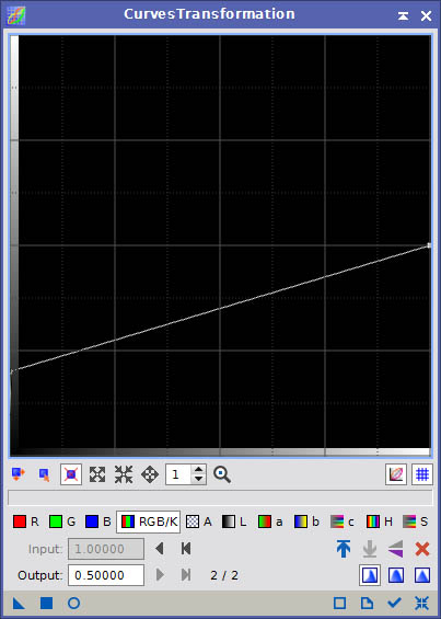Now here is the critical part about creating a good TGV mask. It needs to be low contrast. We want to have higher protection in brighter areas than in darker areas, however it is critical that darker areas are actually protected fairly heavily. This is where manual masking for TGV differs from normal use…we are applying strong protection, and therefor significant attenuation, of the TGV denoising effect to the darker areas. It’s increased protection is what preserves detail and fine grain, while still allowing significant NR. To modify the mask, you need to perform two steps. First, open CurvesTransformation and reset it. Adjust the black point Output level to somewhere between 0.15 and 0.25, for now start with 0.2. Adjust the white point Output level to somewhere between 0.5 and 0.65, for now start with 0.5. Apply CT to your TGV_mask image.

This will brighten the dark parts and darken the light parts, resulting in a lower contrast gray image. We’ve started with 0.2 and 0.5, however in general you will want to tweak these levels depending on the initial contrast of your data…higher contrast data could use more tuning, while lower contrast data could use less tuning.
Once you have reduced the contrast of your TGV_mask, you need to shift it’s midpoint to 50% gray. Open HystogramTransformation, and move the midpoint down until the peak of the histogram reaches the 50% line in the middle. This will brighten the average level of the mask, and improve protection of everything, but particularly the darkest background tones. Now depending on the exact nature of the high frequency noise your image, you may wish to use a slightly brighter or a slightly darker image, with stronger or weaker settings in TGVDenoise. Apply HT to your TGV_mask image.

Low Contrast TGV Mask

You now have both a TGV mask and a Lum mask. You need both. First, apply and invert the TGV_mask to your image. Inversion is important when applying masks to images, as it ensures the brighter parts of the image receive more attenuated NR than darker parts (even though in this case, it’s not a large difference.) Second, expand the Local Support panel of TGVDenoise, and choose your Lum_mask for the Support image. Leave all the other Local Support settings at their defaults. Local support will attune the diffusion process that TGV emulates according to the SNR of the underlying image. Hence the reason a stretched luminance mask is used (by default the I or Intensity component from the HSI color modelization of the image is used, however with linear data, this effectively applies no protection for the majority of the data, excepting stars.) Higher SNR regions of the image receive less diffusion, while lower SNR regions receive greater diffusion.

Before you apply TGV to the image, you should trial-and-error the settings to identify which are best. At it’s default settings, which are usually 5.0 Strength, 0.002 Edge protection, and 2.0 Smoothness, TGV tends to be overpowering and will apply too much NR and diffuse too much across details. I have found that in general, it’s best to reduce the exponent term (the number at the end of the sliders for Strength, Edge protection and Smoothness) for Edge protection to -5 to start, which will protect stars and strong structural details better. You will need to adjust both the exponent and the actual value of Edge protection based on the results of trial-and-error applications.

To properly trial-and-error test a tool like noise reduction in PixInsight, you need to use previews. It is best to draw several previews around key areas in your image. You want to include previews around the following areas:

• Low detail background
• Low detail high SNR
• High structural detail medium SNR
• High star density
• Color-diverse regions

I usually have five to seven preview areas for testing NR in my images. To trial an NR tool, select one of the previews, and apply (drag the small triangle from the lower left of the TGV dialog to the image window). There are two key benefits to doing this. For one, applying TGV to a preview is usually significantly faster than applying to the whole image. Additionally, you an very quickly toggle back and forth between the before and after views of the preview by using CTRL+SHIFT+Z. Trial on one preview and tweak settings for a bit, then iterate through each of the other previews and check/tweak. You want to achieve as much NR as you can without losing either some remnant of the fine grained noise, and without losing fine structural details.

While trialing, use an iteration count of 100. This will speed up the process. When you believe you have found the right settings, increase the iteration count to 500. TGV is a highly iterative process, and while the overall characteristic of the results shouldn’t change a lot when you increase the iteration count, the results should look a bit better and more natural (although the difference will be subtle.) Increase iteration count to 500 and apply to each of your previews just to make sure everything is solid before you apply to the main image. Your results should look something like the following:

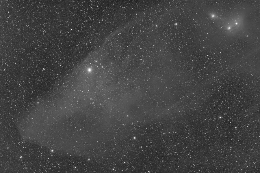
TGV Before and After Comparison

Medium and Low Frequency Noise Reduction

The next linear-phase noise reduction step is to correct medium and lower frequency noise. This kind of noise is a much more difficult form to manage, especially if you are not properly attenuating the NR power. At frequencies lower than pixel level, especially for oversampled data, you begin to run the risk of reducing detail as well. TGV does not handle lower frequencies well, it pretty much just handles the high frequency noise, but it does so very well. For other noise scales, and for additional high frequency NR, we will turn to MultiscaleMedianTransformation, or MMT. MMT is a multi-purpose tool, capable of reducing noise, enhancing detail, and even generating images that represent certain aspects of the image that can be used for custom intermediate processing steps. Like TGV, it is also capable of being run on different channel representations of the image, including RGB/K, Luminance (Y), Lightness (L*), and Chrominance (Cb/Cr). For now, we are going to use it only for NR.

MMT handles noise of different frequencies, or noise of different scales, much better because it is capable of breaking the image up into different layers that each represent a different detail scale. This allows you to be selective about which scales you apply noise reduction to, and to tune the noise reduction for each scale differently. This gives us a lot of power and control over noise reduction at multiple scales. That said, MMT, like most NR tools in PI, is a very powerful noise reduction tool, and without using a proper mask to attenuate it’s effect, applying it effectively without nuking details or plasticizing any given scale can be difficult. Proper masking can again help you preserve detail and fine grain.

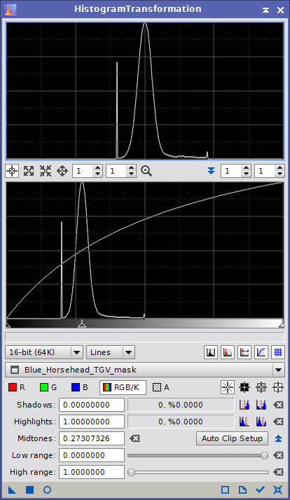
To properly correct the kind of medium frequency artifacts sometimes left behind by TGV, you need to run MMT at a high power for smaller scales, with very high attenuation. This requires a very bright mask in general. Duplicate the Luminance mask you created before for TGV, and open HT. With HT, shift the mid point down such that the histogram peaks somewhere between 70-85%. If your data started out with higher contrast, you may also want to expand the dynamic range expansion tools and expand low dynamic range by -0.5 to -1.0. This will shift all the darker tones up, and reduce the contrast of the mask. You want good protection of the darker tones, and excellent protection of the brighter tones, in your mask. Apply HT to your mask image and rename it by replacing “_Lum_mask_clone” with “MMT_mask”. Your mask should look something like this:

High attenuation MMT mask

Now with a high attenuation mask, we can push MMT to very high power, across multiple scales. Most of the kinds of artifacts that TGV either reveals or introduces are higher-medium frequency. They are not quite single pixel up through several pixels, often a low contrast blotchiness that permeates the image. It’s a subtle effect, but additional processing will usually reveal it more, so we want to correct it. There are also usually lower frequencies of noise, or just artifacts left behind from gradient extraction that take on a bit of a very large scale “ripple pattern”. MMT can also take care of this. Using a technique originally introduced to me by another excellent astrophotographer, David Ault, we will increase the layer count in MMT to the maximum of 8, with the mode set to Dyadic (so the scale of each layer will double from the previous), and we will configure Noise Reduction for each in an inverse ramp to the scale of each layer. Starting with layer 1 and 2 set Threshold to 10, layer 3 to 7-8, layer 4 and 5 to 5, layer 6 to 2.5, and layer 7 and 8 to 2. Leave the Amount at 1.0 for each layer.

Now, depending on your data, you may wish to choose a different Target. We can target Lightness or Luminance, Chrominance or RGB/K. In my experience, if you have a lot of chrominance noise, it is better to target that first before reducing luminace noise further, at any scale. Chrominance noise is an odd duck, and one that often requires care when reducing, as reducing it improperly or too much can nuke the saturation of good and appropriate color as well. DSLR data in my experience tend to have more oddball chrominance noise than CCD data, but a lot of that really depends on how many RGB frames you pick up in addition to L, or how many and how deep your Ha, OIII or SII frames are. It’s possible to go too light on the integration side of things in any case, and end up with a lot of chrominance noise. If you correct luminance first, that can often push high frequency noise down so much that it changes the characteristic of chrominance noise, such that it does not correct the same. So correct chrominance noise first if you need to, then correct luminance. For luminance, I generally choose the CIE Y (true luminance) rather than CIE L* (lightness) option. I do not usually run MMT on the full RGB/K combined data…however YMMV.

As with TGV, you will first need to apply your MMT_Mask, invert it, and then trial MMT on your previews. The main thing with trialing is to make sure the mask is effective enough when running MMT with such high power. Adjust the brightness of the MMT mask small changes to midtones with HT to tune it if necessary. When it comes to both chrominance and luminance MMT NR, you want a fairly subtle effect, however with chrominance it will be particularly subtle. Zooming in to 2:1 or more (I am often at 5:1) can help you discern the differences. You should notice a normalization of color, but you do not want to see a loss of color if you can avoid it. You are unlikely to achieve strong chrominance NR here, you are likely to see some small amount left over, but that is ok. We will run additional chrominance noise reduction passes later on after we have stretched, where the amplitude of the chroma noise increases and is easier to detect, model and remove. You will want at least one pass of luminance reduction here, and depending on the exact nature of your data, how noisy it is, and how much you are attenuating with the mask, you may need more than one pass. With higher levels of noise, attenuating more and running two passes can help preserve more detail and fine grain, although at a slightly greater loss in microcontrast. That is ok, as we can always restore microcontrast with LocalHistogramEqualization (LHE) later on. If you also do chrominance NR here, you may have three total passes with MMT.

Of key importance here is that fine grained noise is preserved, albeit possibly at a lower standard deviation/lower amplitude. You do not want to reduce high frequency noise so much that it basically disappears. You want to keep some. If you have problems with that, you can pull back on the amount for layer 1 (scale 1), and possibly on the threshold as well. You may also try the same with layer 2 (scale 2), but to a lesser degree, if you still have trouble preserving higher frequency grain. With the high frequency grain also goes the microcontrast of finer details, so reduction rather than elimination is very important here. Conversely, correcting the blotchiness that might be left behind by TGV is important. Keep an eye on those higher-medium scale noise frequencies, namely layer 3 and 4. If you are not getting enough correction, you may try increasing the threshold for layer 3 to 8 and layer 5 to 6 to get better correction at those scales. You should quite readily observe correction at those scales in your previews, so knowing whether you need to correct more or not should be a fairly strait forward judgement. When you have it, apply to the image. If you do indeed need to do a second pass for luminance, you may want to scale back all layers. Evaluate the noise at each scale, and either adjust accordingly, or for simplicity you might simply reduce the amount for each layer to 0.75 or 0.5 and try again. In a second pass, I will usually drop the amount for layers 1 and 2 down considerably, to say 0.2, if not lower, in order to preserve those higher frequency details and grain, as the first pass is usually more than enough. Your results should look something like this:

MMT Before and After Comparison (note the reduction in blotching)

It should be noted that I do not reapply STF here. I will keep the STF the same as when I ran TGV, which helps in the evaluation of changes. I will also save off a copy of that STF just in case I for some reason reapply it unintentionally. That said, after I have achieved the NR I want, I will usually reapply STF to stretch the image more. Here is an example of how that once again improves contrast:

MMT After STF

 SERIES

• Part 1 – Overview, NR process introductions, preliminary steps
• Part 2 – Linear noise reduction
• Part 3 – Non-linear noise reduction