Nature Photography

Noise reduction is one of the most fundamental aspects of astrophotography processing. We work with images of minimal signal to noise ratio, a ratio that for best results must be increased, often by a significant amount, in order to produce a quality image. Ironically, given it’s importance, noise reduction is one of the most misunderstood, and possibly one of the least understood, aspects of image processing. PixInsight provides a wide range of powerful noise reduction tools that can assist us in the pursuit of lower noise and higher SNR. These tools are often so powerful, however, that the inevitable result, if you are not already familiar with them (and possibly even if you are) is artifact-ridden, plasticized images that have a very artificial look and feel.

Reducing Noise

The first rule of noise reduction is, it’s noise REDUCTION. All too often, astrophotographers will try to eliminate noise, however this distinction between noise elimination and noise reduction is foundational to good image processing. The goal for you as an image processor should be to reduce the noise in the image. If you eliminate noise, you lose something, one way or another. If you eliminate high frequency per-pixel noise, the data takes on a plastic look, what I call plasticization. If you eliminate lower frequency noise, you are usually going to eliminate some detail as well. Noise reduction is a balancing act, walking the fine line between obliteration and preservation.

Means of reduction

There are two primary ways we can reduce noise. One of these is basically “ideal”, the other is not, but can come close. The first and “ideal” form of noise reduction is the stacking of frames, or the integration of exposure, integration for short. The second, which can be done in many ways, is the application of noise reduction filters. The latter form of noise reduction is something all photographers are familiar with. It shows up as the Noise Reduction sliders in Adobe Lightroom, and similar tools in most other RAW editors. Photoshop has had it’s Reduce Noise, Median and Despeckle filters for ages. This form of noise reduction tends to be “spatial filtering” of one form or another, and tends to redistribute information, which is why it is less than ideal.

If there is one form of noise reduction that I recommend above all others: integration. Stacking more light frames is, in my opinion, the single best way to reduce noise that we have at our disposal. Integrating frames reduces noise “vertically through each pixel stack”, rather than “spatially across pixels.” These two phrases may not mean much to you at the moment, however I am hoping their distinction becomes clear as you continue to read this article. There are risks to data integrity associated with noise reduction filters that are not in play with integration, and if you have the opportunity, gathering more light frames and stacking them will improve your noise in ways that are very hard to approximate with filtering.

There is one additional form of “noise reduction” that we can apply to our images. Basic averaging or multisampling. This occurs when we scale our images down in size. At the most basic level, downsampling an image by a factor of 2, a 50% reduction in width and height, will reduce noise by a factor of 2x relative to the original image. This is because we average together or multisample 2×2 matrices of pixels in the source image for each pixel of the downsampled image. Noise is the square root of the signal, so by combining the signal from four pixels into one, we reduce noise by SQRT(4), or a factor of 2x. Whether this is an effective means of noise reduction or not will really depend on how many pixels you started out with. Most CCD cameras don’t have a lot of pixels, which may render this technique less than ideal unless you prefer to share very small versions of your images. Most DSLRs and mirrorless cameras these days, however, have significant numbers of pixels, usually over 20 megapixels worth, which is usually more than enough to withstand downsampling by a factor of two, and possibly even more (such as with the Nikon D800/D810 or Sony A7r (36.3mp), Sony A7r II (46mp), or Canon 5Ds (50.6mp)).

Cooling for Less Noise

While not actually a form of noise reduction, there is another way we can limit the amount of noise in our data. Electronic sensors, unlike film, suffer from a form of noise that arises due to both temperature and the slow leakage of current through the circuitry of the sensor. This is called dark current, and the amount of dark current tends to increase with temperature. In general, it roughly doubles on average about every 5 degrees Celsius, however exactly what the doubling temperature is depends on the camera, and it can range from as little as 4.5°C to as much as 7°C. Dark current itself is not a noise…it is actually a signal, and as such, can result in an increased offset or separation in your signal if the camera does not employ any kind of dark current removal technology (i.e. CDS, Correlated Double Sampling.) Most CCD and CMOS cameras these days DO employ CDS, which generally means we only get the noise from dark current in our images, but not the offset.

Being a signal, dark current adds noise as the square root of the dark current signal. Dark current is usually measured as a rate of electrons per second per pixel (e-/s/px) at a given temperature. The temperatures used are often 25°C (room temperature), 0°C (freezing), or possibly a sub-freezing temperature in the case of cooled CCD cameras. If the doubling temperature is also supplied, the amount of dark current can be calculated for any temperature. Many cameras today, both CCD and DSLR, have around 0.01 to 0.1 e-/s/px dark current around 0°C. These are reasonable levels of dark current, although not ideal. Some CCD cameras and a very few CMOS cameras have dark current much lower than that, as little as 0.005e-/s/px, at the same temperature. Most DSLR cameras do not use temperature regulation, so dark current can and will vary, often quite considerably, throughout the temperature scale. At higher temperatures, some DSLRs will experience non-linear changes in dark current. In testing, Canon DSLRs often seem to exhibit as much as 8e-/s/px “runaway” dark current over ~30°C, where the amount of dark current starts increasing much faster than the standard doubling rate. At these levels, dark current noise can become the single most significant source of noise in an image, often by a significant margin (i.e. imaging at a dark site, where LP is minimal, dark current noise can be several times more significant.)

Finding ways to reduce camera temperature, particularly for DSLRs as most CCD cameras already include regulated cooling, can produce significant improvements in noise levels during warmer months of the year (which for many places spans half or more of the year.) Camera cold boxes, or even camera base plate coolers (a new type of design that has been experimented with recently, including by myself (articles on my cooler design forthcoming)) can improve dark current levels for DSLR cameras. Additionally, imaging on cooler nights, or finding a cooler region to do your imaging (i.e. away from your city-bound back yard at a dark site, where temperatures can be 10°C or more cooler), can also help improve your results.

“Vertical” Noise Reduction

The stacking of frames, or integration of exposure time, is the means by which we take all of the exposed light from many individual sub exposure frames, and combine them into a single image. As an astrophotographer, you should already be familiar with this, as stacking is a fundamental step for any pre-processing routine, regardless of whether you are using DSS, PixInsight, MaxIm DL or some other tool to do your stacking. You should also already be vaguely familiar with the basic noise reduction power of stacking. Here I’ll be advocating taking this process to the extreme in order to get the most out of the most powerful form of noise reduction we have at our disposal.

We stack in the most basic form by summing the values of each pixel at a given location in each image, then dividing the resulting value by the number of frames we are stacking. In other words, we average our data, pixel by pixel, to approximate the most ideal or “correct” value for each. Technically speaking, this is both strengthening our signal strength, as well as reducing noise. This strengthens our signal because the total amount of light that we gathered across all of our sub frames is combined (summed), producing a larger number in the end. Noise, unlike signal, adds in quadrature, and is therefor the square root of the sum of each pixel added. Therefor, as we add more and more frames, signal increases at a linear rate while noise increases at a decelerating rate:

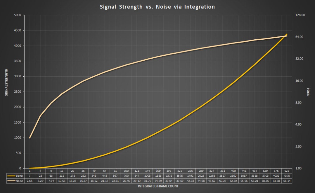
Note: Horizontal (X) axis is logarithmic, but rendered linearly. Signal plot appears curved when it is actually linear, Noise plot has more extreme rise.

From the graph, note that as we continue to stack frames, the increase in noise falls off, while signal continues to grow. When we average the results (which is usually necessary for rendering the combined data into an image), pixel intensity remains roughly the same (but more accurate), each pixel contains more information and also more accurate information, so details are reinforced…and noise is actually reduced:

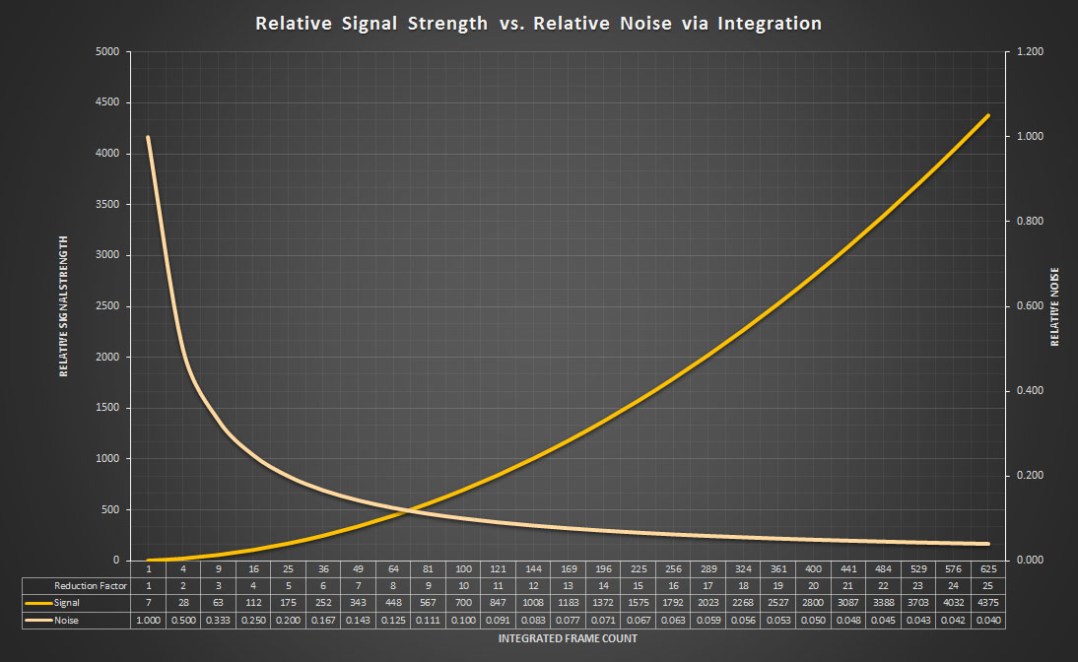
Note: Horizontal (X) axis is logarithmic, but rendered linearly. Signal plot appears curved when it is actually linear, Noise plot has more extreme fall.

Note again that as we continue to stack frames, while we initially see a rapid reduction in noise levels, the relative reduction in noise falls off and eventually flattens. This indicates that there is a definite point of diminishing returns when it comes to integrating exposure for lower noise. This graph runs through every integral “reduction factor” of noise, from 2x through 25x. To reduce noise by a factor of 25x, you need to integrate 625 frames! That is a significant number of frames, beyond what most imagers are either capable of or willing to get, with the exception of those acquired with very short exposures (a minute or less). In my own experience, it is difficult to realize a solid improvement in noise beyond about 300-400 frames without stacking a thousand or more. The only time I would generally recommend integrating more than 400 subs is if you were using very short exposures, such as 15-30 seconds, under heavily light polluted skies. In such a circumstance, it would take a thousand frames anyway to generate an 8-hour integration, which is about the minimum I recommend for a quality integration of light polluted data (it is certainly possible to use less integrated exposure time, however the results tend to lack color fidelity, star quality, and will remain quite noisy).

The one use case where stacking thousands of frames might be viable is video imaging with low noise cameras. Recent advancements in CMOS sensor technology have allowed read noise levels as low as 1e- and in some cases even less. Planetary cameras use high frame rate low noise sensors that are sensitive enough to be used for deep sky imaging by acquiring massive numbers of frames (tens of thousands) at sub-second exposure times, and integrating a significant portion of the best (as much as 75%). This is more of a specialized technique, however it is one of the few cases where vertical noise reduction can produce some incredible results for smaller objects.

Special use cases aside, as much as you can manage it, your first weapon in the noise reduction arena should be to integrate as many frames as possible. This is particularly true in more heavily light polluted areas, where you will be acquiring additional noise from the skyfog signal. Consequently, that additional skyfog signal will usually force you to use shorter exposures anyway, which makes the task of acquiring hundreds of frames easier. At darker imaging sites, especially on warmer nights where you may experience higher dark current, you can still benefit from integrating more frames. In my own dark site imaging endeavors, I have often integrated 80-100 longer exposure frames in the pursuit of very faint details such as IFN or background hydrogen nebula and molecular clouds.

Spatial Noise Reduction

Even with fairly extensive integration, the noise levels in our images can often still be quite high. An interesting fact of SNR in astro images is it is dynamic. It entirely depends on what part of the image you are measuring what your SNR is. Brighter parts of nebula, galaxies/galaxy cores or the cores of star clusters, will all usually have the highest SNR in our images. However these high SNR structures are usually only a small portion of the details that we may wish to reveal in our images. There are fainter details in the arms of galaxies and in outer regions of nebula. There are still fainter details in the often obscuring or distantly reflecting dust lanes. Along the outer reaches of the Milky Way we have some of the faintest details in the sky, Integrated Flux Nebula. The SNR for each of these structures is progressively smaller and smaller. Even with fairly extensive integration, some of these details are bound to be very close to the noise floor, and depending on how much time you have to acquire data, possibly even buried within the noise with an SNR <1:1.

This is where spatial noise reduction filters come into play. By using effective noise reduction such as TGVDenoise, MultiscaleMedianTransformation, etc. we can further reduce the noise in our images and reveal very faint details. Reducing noise in such a manner that we preserve detail while reducing noise is often not as simple as it sounds, and the solutions are often less than obvious. The consequence of uneducated use of PixInsights noise reduction tools is often obliteration…of both noise, as well as structure and detail. The goal of this article is to imbue a proper understanding of PixInsight’s noise reduction tools and how to effectively use them to reduce and preserve, rather than obliterate.

Noise Reduction Phases

There are two primary phases of image processing in PixInsight where noise reduction can occur: linear and non-linear. Within the non-linear phase, there are two primary stages where you may wish to reduce noise, for different fundamental reasons: during stretching, and as part of final processing. Which tools you choose to use in each phase depends on how well they work on linear or non-linear data. While one could probably find a way to use any of the available NR tools in PI to reduce noise in either phase, each tool has it’s strengths. Personally, I prefer the following:

Linear Phase

• Debanding
• TGVDenoise (TGV)
• MultiscaleMedianTransform (MMT)
• Subtractive Chromatic Noise Reduction (SCNR)

Non-Linear Phase

• Adaptive Contrast-Directed Noise Reduction (ACDNR)
• MultiscaleMedianTransform (MMT)
• GREYCstoration (GCS)

If you are familiar with any of these tools, you may notice that my categorizations for when to use them is unusual in a couple cases. For one, many people run TGV on non-linear data, and never on linear data. Some existing PI NR articles advocate the same. Additionally, SCNR is most often used on non-linear data at the end of a processing workflow, even by PixInsight in their processing demonstration videos. I also still use ACDNR, an older NR tool that is no longer recommended as a primary noise reduction tool by the PixInsight engineers, but which still performs very good NR on non-linear data if you know how to use it. Finally, you may notice GREYCstoration listed. This is an NR tool that the PixInsight engineers added some time ago, but which no one quite seems to have figured out how to use. I’ve found it can be a very effective, and naturally adaptive, tool for your final pass of NR over an image after it has been stretched and processed.

While it may surprise most, I often use most if not all of these NR tools on each of my images. The one that may not get any use is GREYCstoration, however I will usually apply the rest to every image, often multiple times. I advocate a multi-stage, multi-pass noise reduction approach with most images due to the fact that processing itself will often reveal additional noise. This is especially true if you like to reveal the faintest details possible, which often requires more extensive processing, particularly more extensive NR to improve the SNR of those faintest details. Luminance noise tends to be easier to manage throughout a complex workflow than chromatic noise. Chromatic noise can take on a variety of forms at a variety of scales, which complicates it’s reduction. Additionally, reducing chroma noise also has the undesirable side effect of damping your color, the fine nuances of which are often quite important for color contrast in fine details.

Noise Reduction Goals

In addition to the two phases of processing where we apply certain kinds of noise reduction, there are specific reasons why we apply noise reduction. Different tools serve goals, and not all noise is the same, nor can all noise be handled by the same tool. There are many kinds of noise that can contribute to the overall noise in an image, and different kinds of noise that  can affect data at different scales. Here is a basic map of which NR tool in PixInsight should be used to deal with certain kinds of noise:

• Horizontal and/or Vertical Banding => CanonBandingReduction (rotate image 90° for vertical banding, then rotate back)
• Well-modeled camera noise => MureDenoise (only works with mono CCD.CMOS data! Incompatible with data that must be demosaiced)
• High frequency/Per pixel noise (luma & chroma) => TGVDenoise, MultiscaleMedianTransform
• Medium frequency noise (luma & chroma) => MultiscaleMedianTransform, ACDNR
• Lower frequency noise (luma & chroma) => MultiscaleMedianTransform
• Inter- and Post-Stretch noise => ACDNR, MultiscaleMedianTransform
• High Chromatic background noise => ACDNR, MultiscaleMedianTransform
• Color-cast from Chromatic noise => SCNR

Using the right tool for the job can be key to achieving the best noise reduction. MMT is a very versatile tool, however it tends to be a bit overpowered, and it usually does not do quite as good a job on high frequency NR as TGV. ACDNR and MMT can often tackle the same types of noise, however sometimes ACDNR actually handles certain kinds better than MMT.

General Techniques

With PixInsight, the “standard” approach to noise reduction is usually less than ideal. Many of PixInsight’s noise reduction tools, like many of their tools in general, include built in masking. Often referred to as either a lightness mask or a linear mask, these masks are often inadequate, and often difficult to understand. Even with the built in masking enabled, most of PixInsight’s noise reduction tools are very powerful, often too powerful, and result in obliteration rather than reduction. This is most often seen with TGVDenoise and ACDNR, both of which are frequently used with inadequate masking and the wrong kind of masks. Even when a mask is generally used with a noise reduction tool, such as a RangeMaks with ACDNR, the range mask applies inadequate protection of darker regions. In both cases, the extreme power of these noise reduction tools, even with generally recommended settings, results in the plasticization of darker image data, which often results in the obliteration of fainter details along with the obliteration of noise.

The crux of effective noise reduction in PixInsight is proper attenuation of the noise reduction effect. Attenuation in this context is the mitigation and proper tapering off noise reduction power. This applies to almost all noise reduction tools in PixInsight, with the two notable exceptions being SCNR and GCS. Attenuation is a fundamental aspect of noise reduction in PixInsight, and not just for brighter pixel data…but all pixel data. This is probably the most fundamental difference between my own approach to noise reduction and most other recommended approaches. With most approaches, attenuation of darker pixel data is almost or entirely non-existent. This forces a reduction in the power of each noise reduction tool, which in turn results in less effective noise reduction in general, not enough in midtoned regions and still too much in darker regions of the image. With proper attenuation, the power of each noise reduction tool can be increased, often quite significantly, attaining more significant reductions in noise. Yet with this increase in power, we are still able to preserve both that pleasing and necessary fine grained structure of high frequency noise, as well as fine details.

The Power of Masking

How do you attenuate an effect in PixInsight? With masking! Masks are probably one of the most under-rated, and yet most critical, functions within PixInsight. As my own skill with PixInsight has increased, I find myself masking for almost everything. I find myself exploring ever more creative was of creating and combining masks, sometimes utilizing ever more complex formulas within PixelMath to produce more effective masks that properly attenuate, in the right regions of the image, the effect of both noise reduction as well as other tools such as HDRMT, HT, ColorSaturation, etc. Masking is the means of attenuation in PixInsight.

More importantly, manually generating proper masks for use with PixInsights noise reduction tools is a far more effective means of attenuating the effect, and allowing clean, powerful noise reduction that preserves fine grain and detail. Manually masking is also the means by which we increase attenuation of darker regions of our images, which are usually woefully under-attenuated with built-in lightness or linear masks. Protection of these dark regions of the image is probably one of the more key aspects of detail and grain preservation. Where a standard RangeMask will usually leave darker regions of an image completely UNPROTECTED, a properly tweaked RangeMask will have the black background level increased by as much as 50%, possibly more depending on the application!

With a proper mask, noise reduction tools can often be run at many times the power (usually the amount or strength setting) that they normally are. Where you may apply MultiscaleMedianTransformation with both lower amounts as well as relatively low thresholds for each layer, with proper masking, you will often find yourself applying MMT with maximum threshold and maximum amount, and possibly some adaptation, for the first several layers, with continued high threshold for additional layers. This kind of power with MMT will usually not only obliterate noise, but it will also usually wipe out both finer scale as well as larger scale details, and on top of that, leave behind severe posterization of the remaining data. Similarly, without proper masking, TGV run at a higher power with higher smoothing will usually leave you with a plasticized background riddled with mid-high frequency noise artifacts, chunky blocks of structure that are basically the remains of both real structural detail and larger jumps in noise levels at the boundaries of that structure. In some cases this artifacting looks somewhat like JPEG compression artifacts. With proper masking, TGV can be run at a very high power with higher smoothing values, which results in very clean reduction in high frequency noise, without totally obliterating it and losing that pleasing high frequency grain that many high quality images maintain.

Prepping your Data

Before we get into actual noise reduction techniques in Part 2 of this series, it is important to make sure you have properly prepared your data. Having the cleanest integrations possible, devoid of the more difficult forms of noise to remove such as hot pixels, banding, and correlated or “walking” noise, helps with the reduction of random noise. Pattern forms of noise are types of noise that we can remove earlier on in our image processing, during the pre-processing and in part even during the acquisition stages. First off, any hot pixels can and should be removed from your individual light frames BEFORE they have been demosaiced, registered and integrated. If you have ideally matched the temperature of your dark frames to your light frames (easy with a temp. regulated CCD, manageable with a cooled DSLR, often unmanageable with an uncooled DSLR), then dark frame calibration should remove the majority of your hot pixels. PixInsight supports something called “dark optimization”, which will scale your dark frames to match your light frames as ideally as possible using high precision noise evaluation.

Bias and Dark Subtraction

For scaling to work, it is important that you generate and use a proper master bias frame. The bias signal is another offset in the image, usually a relatively fixed amount however due to pixel response non-uniformity (PRNU), the bias signal is usually not just a perfect flat offset. It will often contain “glows”, which are small brightened areas either in the corners, or along an edge or edges, which can and usually will show up in your background sky level as you process (particularly once you shift black point to subtract all the various offsets that can shift your signal.) Additionally, particularly in DSLRs, the bias signal is often the source of a lot of banding, particularly vertical banding, in your data, as demonstrated by this 512-frame master bias image:

512-frame Master Bias Signal

So it is best to actually generate and utilize a master bias, or a superbias (which is a bias frame produced by removing all the noise from a master bias image), and use that to remove this signal from all of your frames, including dark, flat and light frames. In the case of a master dark frame, you may start out with data that has both horizontal and vertical banding (and possibly additional glows, another key reason to use dark subtraction) such as this master dark frame:

20-frame 30-minute Master Dark Frame (Uncalibrated)

After subtracting away the master bias, you should find that the majority of the vertical banding is now gone:

20-frame 30-minute Master Dark Frame (Calibrated)

Once the bias signal has been properly removed, you will have data that contains only image signal and noise. This is critical when performing things like dark optimization (which scales darks) and flat normalization (which scales flats), as without removal of the bias signal first, it ends up being larger or smaller in the darks and/or flats than in the lights, and subsequent subtraction or division of those master calibration frames results in incorrect calibration. Removal of the offsets normalizes the data allowing for proper scaling. For reference, here is the above bias-calibrated 30-minute master dark after being scaled to a 90-second light:

20-frame 30-minute Master Dark Frame (Calibrated and Scaled, K = 0.05)

Note the near-absence of noise in the scaled frame. One of the benefits of using long scaled darks is you can use few individual frames (I usually use 10 to 20, rather than around 50) and have a lower standard deviation of noise in the scaled dark, which has a statistically meaningless impact on the standard deviation of noise in the calibrated light. The only real caveat with scaled darks is glows tend to grow at different rates than hot pixels, as the source of heat causing them is usually different. If you have amplifier glows or any other glow in your darks, it is still best to keep your dark exposure lengths the same as your lights. The scaling factor, K, will then be closer to 1.0, and thus glows will be properly corrected when the dark is subtracted from the light.

Cosmetic Correction

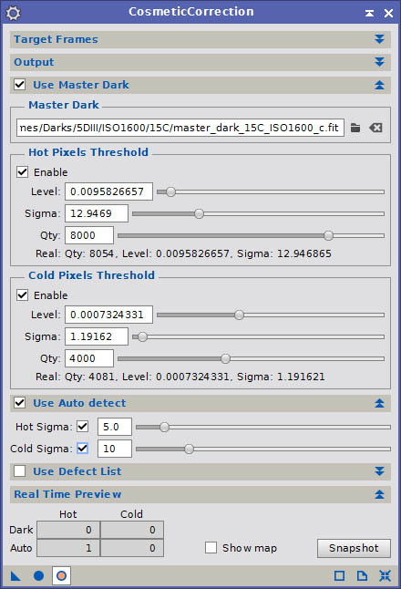
Cosmetic Correction Dialog

Sometimes stuck and hot pixels don’t actually get properly handled by dark frames, and if you are using dark scaling with a master dark too far removed in temperature from your lights, you may experience some remnant hot pixel data in your frame. You may also not even want to bother with dark subtraction if you have higher noise levels in your dark frame, as subtracting random from random gives you even more random (in other words, your standard deviation increases when subtracting noisy master dark frames). PixInsight has another tool called CosmeticCorrection which can help you identify and correct hot and cold pixels via several means: Master Dark Pixel Mapping, Automatic Detection over Sigma, and via a Defect Map listing. After running a good cosmetic correction on your light frames, they should end up “pristine”…completely devoid of any major deviant pixels.

You may ask, why bother? If you have enough hot pixels, especially if they end up demosaicing to larger multi-pixel blobs or crosses, they can affect image registration by being detected as stars. I have expereinced this myself on a few occasions, and assisted several astrophotographers who have experienced similar issues. The results often look like either severe chromatic aberration (which is really a color shift across the frame due to the fact that alignment occurred on hot pixels rather than the stars, yet the offset from ideal is small), or stuttered star trailing. This issue can often be corrected by adjusting registration parameters, however with enough hot pixels, even with noise reduction, they can still end up becoming primary registration points.

If you do not have registration issues, the other potential issue is leaving hot pixels in your frames for integration. It is possible to correct outlier pixels by using dithering and sigma-rejection algorithms when integrating. However this requires dithering, and with sensors that use a color filter array, dithering must usually be quite aggressive in order for the entirety of a demosaiced hot pixel to be identified and rejected by an algorithm such as Winsorized Sigma Clipping. Very aggressive dithering tends to add a significant amount of imaging time overhead, as it can take a minute or two between each frame to properly offset the star and reposition.

I personally advocate a simpler and faster approach to dithering, one of moderate aggression, with smaller offsets that requires less recovery time (often as little as 10 seconds). I also advocate dithering only between every 2-3 frames unless you are using very long exposures and will be integrating 20 or fewer lights. Dithering is still an important aspect of imaging, as it eliminates the possibility of correlated noise showing up in your integrations, and it offsets stars enough that you can drizzle the integration to improve sampling and/or resolution. However with moderated dithering, you can gather more light frames each night, since you will only be wasting seconds between every couple of frames, rather than minutes between every frame. A moderated approach to dithering can diminish the effectiveness of sigma rejection during integration. This can leave behind demosaiced hot pixels, which in my experience often behave as loci for noise reduction artifacts. They can also act as loci for artifacts from other tools, such as deconvolution (often severe dark ringing), star reduction, contrast enhancement, etc. I find it is important to totally eliminate all hot pixels before processing to avoid any of these artifacts.

The simplest way to apply cosmetic correction is simply to generate a Master Dark frame, reference it, and adjust the Qty (quantity) setting for hot and cold pixels to identify and remove them. You can check to see which pixels are being identified in your image by enabling the real time preview, then enabling the Show map option in the Real Time Preview panel of the CosmeticCorrection dialog. You can click the Snapshot button to generate an image where any identified hot pixel in your image matched a mapped hot pixel in the master dark. Adjust the quantity for hot and cold pixels to identify more or less as appropriate for your data. If you are concerned about increasing noise by subtracting a master dark frame¹, then Cosmetic Correction can correct most hot pixels without any dark subtraction at all.

For some images, if dark frame subtraction worked well, you may not need to use a master dark as a hot/cold pixel reference. In such cases, you could use only Auto Detect, which will identify any pixels in the image that deviate from the median level of their neighbors by more than the specified Sigma (σ), and replace it with the median of it’s neighbors. Auto detection can work wonders, however you often have to be careful about the sigma value you choose. Too low, particularly for hot pixels, and you run the risk of identifying some star halo pixels as deviants, and they will be replaced. This can result in visible degradation of some star halos. In my experience, a sigma of 10-12 is often about the lower limit for my data. You will need to experiment to identify the best sigma for your data.

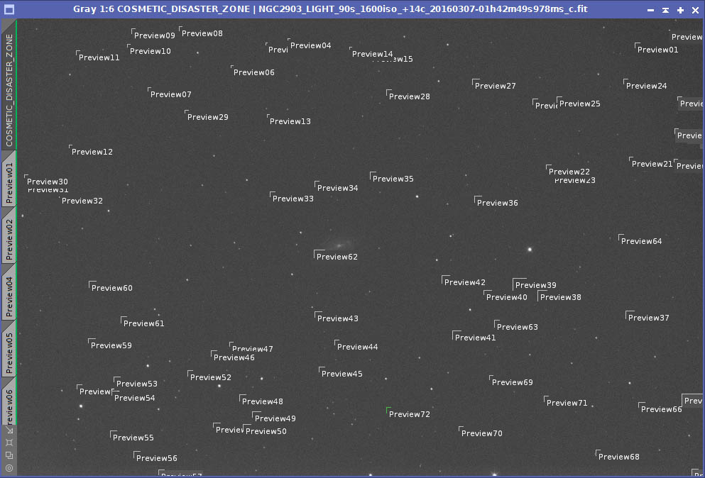
Cosmetic Disaster Zone: Previews drawn around major hot pixels in a light frame

The third option for identifying hot and cold pixels for correction with CosmeticCorrection is to use a Defect List. A defect list is a manually created map of all deviant pixels that you wish to correct. Persinally, I find the defect map, used in combination with a high-sigma Auto Detect, is usually the best solution. This is due to the fact that, for some reason beyond my understanding, neither dark subtraction, master dark reference, and auto detect seem to detect ALL hot pixels in my average data. I don’t have a terrible lot of these pixels, however there are a few, and they tend to be quite intense and often positioned such that they produce the most egregious knots of red, blue, and green after the frames have been demosaiced. The best way to identify and map these pixels in a defect list is to draw a small preview (larger than 13×13 pixels) around each hot pixel in a single light frame, as in the screenshot above.

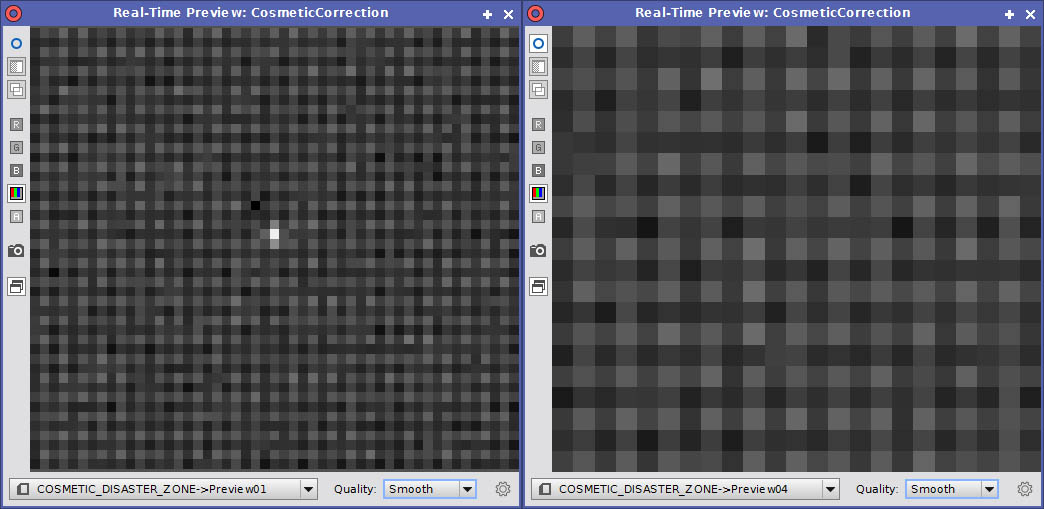
Identification of automatic hot pixel correction

Once you have identified each hot pixel and drawn a preview around then, BEFORE adding any to the defect list, you will first want to enable the real time preview. You will also want to enable the master dark and/or auto detect features, whichever you intend to use with defect list. IFfyou are working with mosaiced data, you will also want to enable the CFA option in the Output panel of the CosmeticCorrection dialog, as this will ensure that the hot and cold pixels are replaced with the medians of LIKE-colored pixels. Scan through each of your image previews in the real time preview. The master dark and/or auto detect should identify and eliminate most of the hot pixels you identified. For those that have been corrected (right side of the examples above), remove those previews. For those that have not, keep those previews. After you have eliminated all of the previews for automatically corrected pixels, you can easily go through and map out the pixels from the remaining previews. Note that it is very important that you do this mapping on the full image, NOT on a preview…otherwise the detected coordinates will be incorrect. I usually add pixels by row, with the Limit option enabled. The limit will be by column if using row, or by row if using column. Simply click the center of a hot pixel to identify it’s row and the row and limit will be set automatically. Then click the Add defect button.

Once you have identified all deviant pixels, save your defect list out. This can be reused over and over for subsequent calibrations, and you may periodically find the need to add new pixels to it that are not caught by the other two removal methods. From this point on, cosmetic correction of your images should be very quick and easy, resulting in pristine light frames for subsequent registration and integration. At this point, you have the cleanest light frames you can get. The primary form of noise left in the images is random noise, which will be reduced further by integrating, and which is easy to deal with when performing spatial noise reduction. You should now demosaic, filter (either with Blink, or SubframeSelector, etc.), register, and integrate your light frames. Once you have the final integration, you can move onto part to of this article for an explanation of how to most effectively apply TGV, MMT, ACDNR and GCS.

SERIES

• Part 1 – Overview, NR process introductions, preliminary steps
• Part 2 – Linear noise reduction
• Part 3 – Non-linear noise reduction