Nature Photography

When it comes to getting quality results with astrophotography, in the end one of the primary concerns is SNR. Signal to noise ratio is one of the primary things that affects the quality of an image (one of the primary things…however not the only thing, I’ll cover others in additional articles.) There are a number of noise sources that reduce the SNR if our images, some of which are well known, and others which are not quite so obvious. The common ones that most should know are read noise (probably the most well known), dark current, and the signal itself.

Every signal has an intrinsic noise. We call this photon shot noise, which follows a Poisson distribution. The thing that may not be as well known is that a signal isn’t just a signal…sometimes we gather signal from multiple sources, when we really only want the signal from one of those sources. With astrophotography, the primary sources of signal are the light from space itself, light from “airglow” in the atmosphere, and light from artificial light sources reflecting off the atmosphere (light pollution.) We care about the light from space…however any additional light is unwanted, an additional source of noise, and ultimately a drag on achieving the kind of high SNR required to produce the best images.

DEFINING SNR

The most basic signal to noise ratio formula is as follows:

Where S is the signal and N is the noise. The noise itself in a pure signal is:

Which means our SNR formula is really:

This simplistic formula doesn’t really tell us the whole story, as the signal is only one of the potential sources of noise. Additionally, it is important that we differentiate the various signals, and determine our SNR relative to only the signal we are actually interested in keeping.

ACCOUNTING FOR ELECTRONIC NOISE

Because a digital camera is imperfect, we cannot simply assume that the only noise in our image is SQRT(S). We have to account for additional sources of electronic noise, such as read noise and dark current:

Dark current and read noise are different in nature. One of them, read noise, is actually a constant term for a given camera and gain/ISO setting. When imaging at a given gain/ISO, the same amount of read noise will be added to every sub exposure frame you acquire. This is an important trait, one that can impact stacking and sub length, that I’ll cover later in this article.

Dark current is also a source of noise in our images. Intriguingly, dark current is also a signal. It is a slow and steady accumulation of charge in the pixels due to leakage current, which varies with heat. Without anything to suppress it, a long enough dark frame exposure would eventually clip out to pure white, as that slow accumulation of charge would eventually saturate the pixels. However due to the way modern sensors (both CCD and CMOS) are designed, we usually don’t see this signal, usually called an offset, nor do we have to deal with it. Dark current itself is suppressed via technology called CDS, or Correlated Double Sampling. Being a signal, like any other, it has it’s own noise:

While the sensor circuitry will remove the dark current offset for us, it’s noise cannot be removed. That noise will show up as increased random noise relative to the square root of the dark current, and it will show up as hot pixels, as each pixel will respond to leakage current a little differently. Most pixels will experience the average amount of current leakage, some will experience a little less or a little more, and a few will experience significantly less or significantly more. This leads to hot and cold pixels, and is the primary reason we use dark frame subtraction.

FACTORING IN UNWANTED SIGNALS

In addition to the dark current and read noise, there is another potential source of noise. This source of noise is often the most egregious, adding significantly more than read noise and often more than dark current (especially with newer low dark current cameras like most Sony Exmor based cameras, the 7D II, etc.) This additional source of noise is light pollution. Light pollution is a source of additional photons entering the telescope (or camera lens) and reaching the sensor. Over time, the total signal in each pixel of the camera will increase because of both the photons reaching it from space, and the photons reaching it from light pollution.

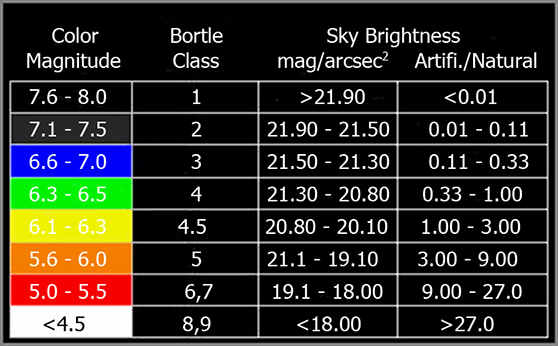
In a city, light pollution is usually the most significant source of photons, often by a significant multuple. The average suburban home tends to be in a red zone on the Bortle scale, where light pollution flux (usually called skyfog flux) may be 9-27x higher than the flux from the object in space (usually called object flux…a flux here is the flow of photons.) That means that if your object in space is capable of delivering say 20 photons per minute to each pixel, then skyfog would be delivering 180-540 photons per minute to each pixel.

Away from the city, in rural areas where the density of artificial light sources drops considerably, skyfog flux may be as little as 0.1-0.5x the object flux. If your object flux is 20 photons per minute, then your skyfog flux would be 2-10 photons per minute. This useful chart gives you a rough gauge of artificial light to natural light (skyfog to object flux) ratio, depending on the Bortle Scale zone your imaging in:

LIGHT POLLUTION AND IT’S NOISE

Since light pollution, or skyfog, is a signal, it has noise:

In the city, since the skyfog signal can be so significant, and often many times more significant than your object signal, it tends to have a lot of noise. For example, in our previous hypothetical scenario where the object flux was 20 photons per minute and the skyfog flux was 9-27 times higher than that, the noise from skyfog would be as much as:

Out of context that number, 23.27, may not mean much. So let’s put it in context. Let’s assume for the moment that our camera has 100% Q.E., which means our skyfog noise is 23.27e-. Your average read noise in a DSLR at a higher ISO of 800-1600, common settings for astrophotography, is likely to be anywhere from 2-5e-. On an average night, the dark current in a modern DSLR might average around 0.02e-/s/px, meaning in a five minute sub exposure, your dark current noise is:

Furthermore, out object signal itself was only 20e-, which means it’s noise is only 4.47e-. With all these numbers, it should be easy to tell which one is adding the most noise to the image:

The light pollution has added the most noise by a significant margin. It has also added a relatively strong signal as well, and here is why this source of noise is often the most insidious kind. If you look at a stack of sub frames strait out of a tool like DSS, you will usually see the background as a light brownish gray color, the whole image will appear as though it has a kind of haze over it. It will seem as though your actual deep space object, say the Pleiades or Andromeda Galaxy, resides “behind” this layer of haze.

Well, in actuality, that is exactly the case! 😉 The haze is in Earths atmosphere, and your DSO does indeed sit distantly behind it. However, we can correct this issue by removing the light pollution signal. The simplest way we do this is by offsetting it, or subtracting it out, by shifting the black point of the image up. Here is the insidious part: While a signal can be subtracted out of an image…it’s noise cannot be. When you subtract out the light pollution signal, it will still leave behind it’s noise.

THE FULL FORMULA

Now, total noise in an image is not simply the linear addition of all noise terms. Noise adds in quadrature, because all the separate noise terms are first added, then the square root of that entire sum is taken. Here is our full SNR formula:

Notice the fact that the skyfog signal is in the noise term, but not in the signal term. We are uninterested in the skyfog signal…the only signal we are interested in is the object signal. However since we cannot remove the noise from skyfog, it must remain a part of the noise term.

If we use our previous object and skyfog flux levels with a two minute exposure (again, assuming we have a 100% Q.E. for simplicity sake), we would have 40e- object signal and a 1080e- skyfog signal. With a dark current rate of 0.02e-/s/px, our two minute sub exposure would have 2.4e- dark current. Let’s assume ISO 1600 with read noise of 3e-:

Well that is a rather uninspiring ratio. 😉 It’s barely more than a 1:1 ratio, which means the DSO details are mostly buried within the noise. You want a ratio closer to 5:1 at the least, and the higher you can get it the better.

STACKING & SIGNAL INTEGRATION

So how does one improve their SNR? Well, the first and most basic means is by stacking. Stacking images integrates all the information from each image and produces a single output image with higher SNR. The amount of noise reduction you get from stacking is the square root of the number of individual sub frames stacked. If you stack two sub frames, you reduce noise by a factor of 1.4x, if you stack 4 frames you reduce noise by 2x, 9 frames reduce by 3x, 16 frames reduce by 4x, 25 frames reduce by 5x, 64 frames reduce by 8x and 100 frames reduce by 10x.

This can be calculated using a tweaked form of our SNR formula:

If we stacked 100 of our previous hypothetical frames:

That is a better SNR, something definitely usable. It is still not ideal, but it will give you a more workable signal and you’ll be able to make a nice image of it. It did require a rather significant 100 subs to achieve, however, and that is only for a moderately brighter object. For fainter objects, the SNR will only get smaller.

Stacking can effectively provide continuous gains, at least so far as truly random noise is concerned. So long as you are willing to keep acquiring light frames, more stacking will continue to reveal fainter details. The value of stacking has a certain amount of diminishing returns, as to reveal details half as bright you must stack four times as many frames. So, if you’ve stacked 64 frames, and need to reveal details half as bright, you would need to stack 256 frames. If you still need to reveal details half as bright as stacking 256 subs reveal, you would need to stack 1024 subs, etc.

Another potential source of diminishing returns is correlated or stacked patterns during integration. If you have not properly calibrated and cleaned up the pattern noises, stacking will eventually reveal them, just like any other fixed structure in your signal. Proper calibration is key to getting the most out of stacking.

These differences bear out visually in stretched results. The table below demonstrates how much stacking can reduce noise and improve the visibility of faint details.

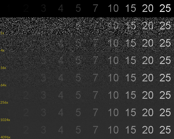
The top row demonstrates an original signal, with details fading in intensity. The second row demonstrates a single “sub” where the number 10 has an SNR of 1:1. The subsequent rows represent the benefits of stacking 4, 16, 64, 256, 1024 and 4096 subs. By the time you have stacked 16 subs, there is little continued benefit to the number 25. Noise does drop further with additional stacking, but to little effect from a visual or SNR standpoint. However, the number 10 continues to improve up through stacking 64 subs. Additionally, the number 1 does not even show up at all until you have stacked at least 64 subs, and only becomes well-separated from the background noise by 1024 subs. The number one becomes clean with a good SNR by 4096 subs.

How much you stack depends a lot on how faint the details you are trying to reveal are. If you cannot reveal your target details with fewer subs, then you will need to acquire more. Stacking is one way to integrate exposure time to increase signal strength. However using longer exposures is also another way to increase integration time. So long as you are not exposing too long, and thus needlessly wasting dynamic range, it is generally better to expose for longer first, before increasing how many subs you are stacking. Once you have reached a reasonable limit on exposure time, then the best way to improve SNR is by stacking, as exposing longer or stacking will produce roughly the same SNR in the end, whithout the risks inherent in even longer subs (such as sub losses due to environmental factors like wind, frame intrusions like satellites, airplanes and meteors, tracking issues, etc.)

THE VALUE OF FILTERS & DARK SKIES

So how do you improve your SNR? According to the math, light pollution in a suburban back yard near a metropolitan city area is by far the single most significant source of noise. So the simplest way to improve SNR is to reduce light pollution. That can be done in a couple of ways. One is to use a filter of one kind or another to block light pollution. There are pros and cons to that option, which I’ll get into in a moment here. The other option is to go to a location that doesn’t have as much light pollution. That also has it’s pros and cons, although if you really want to get the best results, it tends to be the best option despite the cons.

LP Filters

Filters are probably the simplest way to improve your SNR without having to move to a different imaging location. There are a wide range of filters that can reduce skyfog flux, and some are better at it than others. Which kind of filter you use will partly be determined by the kind of camera you are using, and partly determined by what kind of results you want. If imaging with a DSLR, you will want to look into light pollution (LP) filters. There are a variety of kinds of LP filters, each with a different bandpass that supports certain kinds of imaging. The primary LP filters to look into are the IDAS LPS-P2, the IDAS-V4 or Astronomik CLS, and various UHC (ultra high contrast) filters.

The IDAS LPS-P2 (or LPS-D1 if your using an astro-modded DSLR, or alternatively the Orion SkyGlow Astrophotography filter) is a multi-bandpass LP filter designed to filter out the most egregious sources, namely Sodium and Mercury vapor lighting, most commonly used in street lamps within urban and suburban areas. This kind of filter does not block out as much LP, but it preserves more of the green range of the spectrum which supports better color balance. It will filter enough light to give you about a stop and a third or so additional exposure time.

The IDAS LPS-V4 (and also the Astronomik CLS and Orion SkyGlow Broadband filters) is a “broadband” filter. Unlike the LPS-P2 which passes many bands across the full visible spectrum, the LPS-V4 blocks most of the spectrum and only passes two broad bands, one around the blues and blue-greens, and one around the reds. This filter blocks most of the greens and yellows, which has a more significant impact on color balance…however as it blocks out more light pollution, and will offer about two stops or so of additional exposure time for even higher contrast. These filters are often called nebular filters, as they tend to give better exposure on emission nebula (oxygen, hydrogen, sulfur and nitrogen gas nebula).

Finally there are also UHC filters, which are similar in design to the LPS-V4, but with narrower band passes around the blues and reds (primarily becoming oxygen and hydrogen nebula filters). They allow even longer exposures for even higher contrast.

The biggest benefit of using an lp filter is that you don’t have to pack up your gear and haul it out of the city to do any imaging. This makes them extremely convenient, and as they are relatively cheap ($80-$190), a very cost effective way to start getting better results from your suburban back yard, or even a park near the city. The primary drawback is that they filter light, and that has an impact on overall color quality. Depending on the exact nature of the filter, it can also impact other aspects of image quality, including star quality, noise characteristics, etc. Every individual will have different tolerance for these potential issues, and if you are just wetting your feet with astrophotography, they are usually the best way to start getting better SNR…and thus better results…with your imaging. LP filters will usually not give you the most ideal results, however, and you may wish to resort to the more effective options below.

NARROW BAND FILTERS

Imaging with a DSLR is a great way to get started with astrophotography, however you will eventually run into the limitations inherent with such equipment. Even with LP filters, there is only so much quality you can extract from a DSLR. A DSLR camera (or mirrorless camera) uses a color sensor. Color senors usually have some kind of color filter array over the pixels, usually a “bayer” filter array. This implicitly restricts the amount of light that can be sensed at any given pixel to around 30-40% (depending on the exact characteristics and bandpass of the red, green and blue filters). Combined with the often more limited quantum efficiency of a DSLR, overall sensitivity of this kind of camera is quite low, and a relatively inefficient means of acquiring signal and maximizing SNR.

A more efficient means is to use narrow band filters. This requires the use of a monochrome camera, usually a CCD. A good narrow band filter, with an appropriately narrow bandpass to filter out the most light pollution and support the longest exposures, can cost anywhere from approximately $200 to $600 or even over $1000, depending on the size. For most use cases, you should expect to spend somewhere between $300-$500 on a good narrow band filter with less than a 7nm bandpass. The narrower the band pass, the more light will be filtered out, and the greater the contrast you can get on the desired frequency of light. With narrow band filters, you can effectively filter out all light pollution, and in some cases, even filter out most moonlight.

There are several common bands that are frequently used in astrophotography. The most common of these is Ha, or Hydrogen-alpha. This is a reddish emission from hydrogen nebula, which is quite prolific in space, and is usually the easiest narrow band data to acquire. Hydrogen tends to be more structured than other gasses, and is often used in place of or as a compliment to a luminance filter with LRGB imaging. The next most common is OIII, or Oxygen III. This is a greenish-blue emission from oxygen nebula, which is less common than hydrogen, but common enough that it is usually the second choice for bi-color narrow band images. Oxygen is usually more diffuse than hydrogen, cloudy, translucent and wispy with less defined structure. Another common filter is SII, or Sulfur II. This is a deep red emission, a darker and deeper red than hydrogen. It is also more uncommon than hydrogen, some targets lack any significant sulfur, while others have quite a bit. SII is usually used to make tri-color or “Hubble Palette” images, where Ha is mapped to green, OIII is mapped to blue, and SII is mapped to red. The last somewhat common narrow band filter is NII, or Nitrogen II. This is another reddish emission about the same color as Ha, but is most often found in planetary nebulas, and not in too many others. It is often mapped to red or green, or a combination of the two, and in some cases it is mapped to blue.

With narrow band filters, you will require very long exposures, as the filter passes such a minimal amount of light. Shorter narrow band exposures are usually around 15 minutes, but more commonly 20-30 minutes, with longer exposures of 45, 60 and even as much as 90 minutes for particularly faint objects. That is PER SUB, and total integration times are usually measured in the many hours, usually 10-20 hours and up. Despite the need for long exposures and long integration time, narrow band imaging delivers excellent results with superior quality, and can be done from just about anywhere, even the average suburban back yard. With automation software, the imaging process can be done unattended in many cases, which greatly eases the process of acquiring the necessary data.

If your looking for the best results with backyard imaging in the city, narrow band with a CCD will deliver significantly higher SNR’s than any other option in most cases.

DARK SKIES

The final option for getting better results, which is useful whether you use a DSLR or a CCD camera, is to use a dark site. Light pollution exists overhead in cities, however all it takes is a drive out to a nearby rural area to find considerably darker skies. Anyone who has done astronomical observing for any amount of time will recognize the term “dark site”, and that will likely evoke memories of very long drives to extremely remote locations. For the best visual observing, such a trip is usually a necessity, as the sensitivity of the human eye is dynamic. The proximity of a light pollution “bubble” from a nearby city will limit how good your dark vision gets, which will in turn limit how much you can see in the sky unaided, with binoculars, or with a telescope. A DSLR or CCD camera, on the other hand, has fixed sensitivity. The proximity of a light pollution bubble has no secondary impact on the camera’s ability to gather light from whatever it’s pointed at. As a beneficial consequence, you can usually find a good “imaging dark site” within a much closer distance from an urban or suburban area than a good “visual observing dark site.”

My own most-used dark site is a mere 35 minutes from home, out in a nearby rural area to the east of Denver, CO. The image above of my preferred light pollution map shows the location of my dark site relative to the greater Denver region. Any area on this map that is cyan or darker makes for an excellent imaging dark site. Green is still good, yellow is decent, but you will still have to deal with a fair amount of light pollution in a yellow area. Orange, red an white, and you will have to deal with significant amounts of light pollution. You really want to find a cyan region, where the percentage of total signal that is artificial is smaller than the percentage of total signal that is from your DSO (deep space object). In a region like this, image quality without any filters will improve across the board…higher SNR, richer color, greater contrast.

As with narrow band filters, you will find that you can and generally should use longer sub exposures at a dark site. You won’t need (or even be able to use) 15 minute or longer exposures, however don’t be surprised if you need at least five minutes, if not eight, ten, even twelve minutes at a very good dark site (gray or black zone.) As with narrow band filters, longer exposures under darker skies take longer to reach the ideal exposure point (i.e. 1/4-1/3rd from the left on the back of camera DSLR histogram), which means the contrast and SNR in each and every sub is higher, often significantly higher, than a single subs from a light polluted zone. Stacking 16 or more of these kinds of subs will result very good SNR for either DSLR imaging or LRGB filtered imaging with a monochrome CCD.

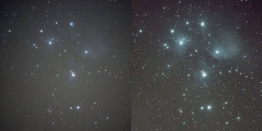
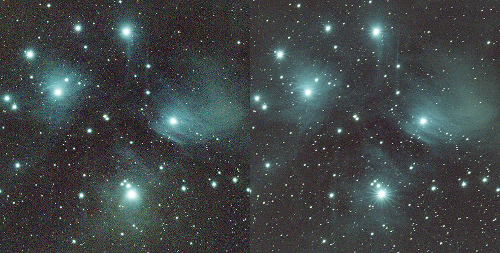
Light Polluted vs. Dark Site – Single Sub Exposure – LP Subtracted: 18.7mag/sq” Suburban Site (Left) – 21.3mag/sq” Dark Site (Right)

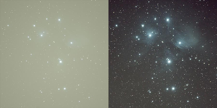
Another benefit of using a dark site is that you can better use your camera’s dynamic range. The Pleiades images above demonstrates this. While getting the longest exposure possible (till 1/4-1/3rd histogram) at a dark site is ideal, some objects have a lot more intrinsic contrast, and shorter subs are necessary. The Pleiades images above are identical single frame exposures, one taken from my red zone back yard (measuring ~18.7mag/sq” that night) and the other taken from my primary dark site (measuring ~21.3mag/sq” that night). In the first comparison, the image from my back yard has been stretched identically to the dark site image, without offsetting the light pollution signal. In the second comparison, the light pollution signal has been subtracted out. Note the significantly brighter background sky in the first version of the light polluted version of the image. Note the increase in contrast with the dark site image, relative even to the light pollution version after the light pollution has been subtracted out, and also note that the stars are exposed to roughly the same levels. The Pleiades is a cluster of very bright stars, and clipping them is generally a necessity in order to get sufficient SNR on the nebula structure. At a dark site the background sky level is a good deal darker, revealing both more nebulosity as well as an increased number of fainter stars. Another challenging bright object that is easier to image at a dark site is Orion Nebula, which may represent as much as 18 stops of dynamic range.

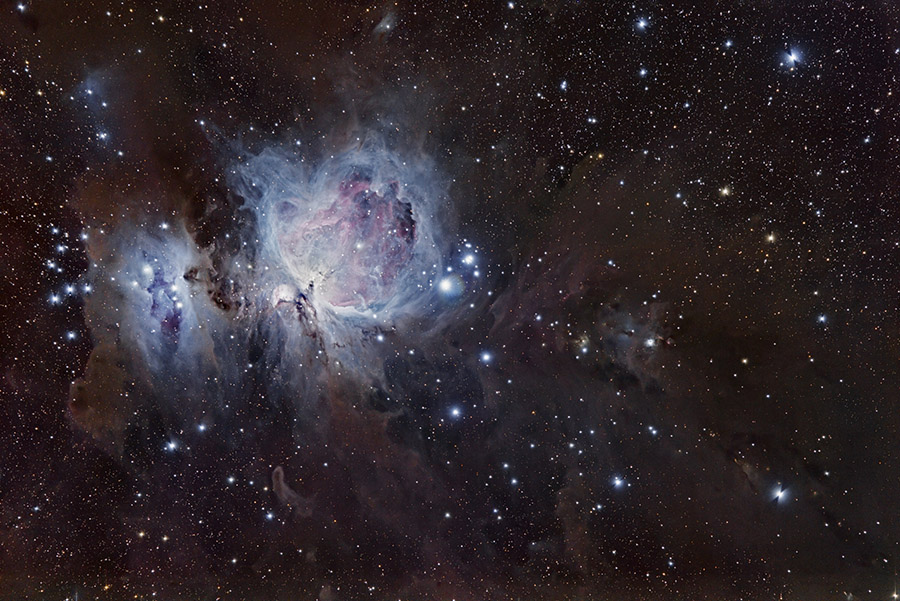
Orion’s Sword – HDR – 2h20m Dark Site Integration (~17-18 stops dynamic range with HDR Composition of 7 separate integrations graded down by full stops)

COMPOUNDING READ NOISE

There is one final caveat about read noise that should be understood. Read noise is a type of noise that is added to an image as the signal is read out and converted from analog to digital. There are usually a number of sources in the circuitry of a sensor and it’s readout logic that can add noise to the image signal, and generally manufacturers lump them all together as an RMS (root mean square) called “read noise”. Since this noise is already denoted as an RMS, it must be squared in the noise term of our SNR formula. The reason for this may become more clear if we make the noise term an RMS itself:

Noise is the square root of a signal:

We can always calculate SNR, even if we don’t know all the signals, but do know their noises. This can be useful when deriving dark current from the dark current noise present in an image that was produced from a sensor that uses CDS. The CDS unit will remove the dark current itself, leaving behind only it’s noise…but the noise is the square root of the dark current. So we can simply square it to determine the original signal. Hence the reason a noise that comes from multiple sources is a Root Mean Square:

We square read noise because it is an RMS itself. This presents an interesting conundrum for stacking. Since read noise is a constant addition to any exposure, regardless of the exposure length, when we combine multiple subs, the read noise compounds more:

Squaring the read noise term can make it much larger, especially if it is not a particularly small single-digit number to start with. Read noise of 3e- squares to 9e-, read noise of 4e- squares to 16e-, read noise of 5e- squares to 25e-. Read noise of 25e-, not uncommon in a Canon DSLR at lower ISO, squares to a whopping 625e-! When it comes to stacking, it is best to stack as few subs as possible. This is especially true if your read noise is higher…from about 5e- RN onwards, read noise will start to have a more significant hit to SNR as you stack more shorter subs. Using filters or a dark site will allow you to expose longer than you could unfiltered in a light polluted zone, which will reduce your sub count, and thus reduce your total read noise. If you are used to using 30-60 second sub exposures in a red zone back yard, and move to a dark site, it is best to find the longest exposures you can get away with, without your histogram peak going past 1/4 to 1/3rd from the left. That should increase the contrast of details in each and every sub, reduce sub count…possibly quite significantly, and thus minimize the amount of total read noise that ends up in your final integration.

It is not unheard of to use 256 subs or more from a light polluted zone, even with a light pollution filter. (I myself have integrated upwards of 260 subs on occasion for fainter details in certain objects.) A significant reduction in sub count can be realized by moving to a dark site, where you may need as little as a mere 16 subs that are two, three, maybe even four times longer than your light polluted subs. Even if you do end up needing more sub exposures at a dark site, you will usually find that you rarely need to go into the hundreds, and will usually not need to go beyond 64 if you are able to get deep enough exposures on each sub.

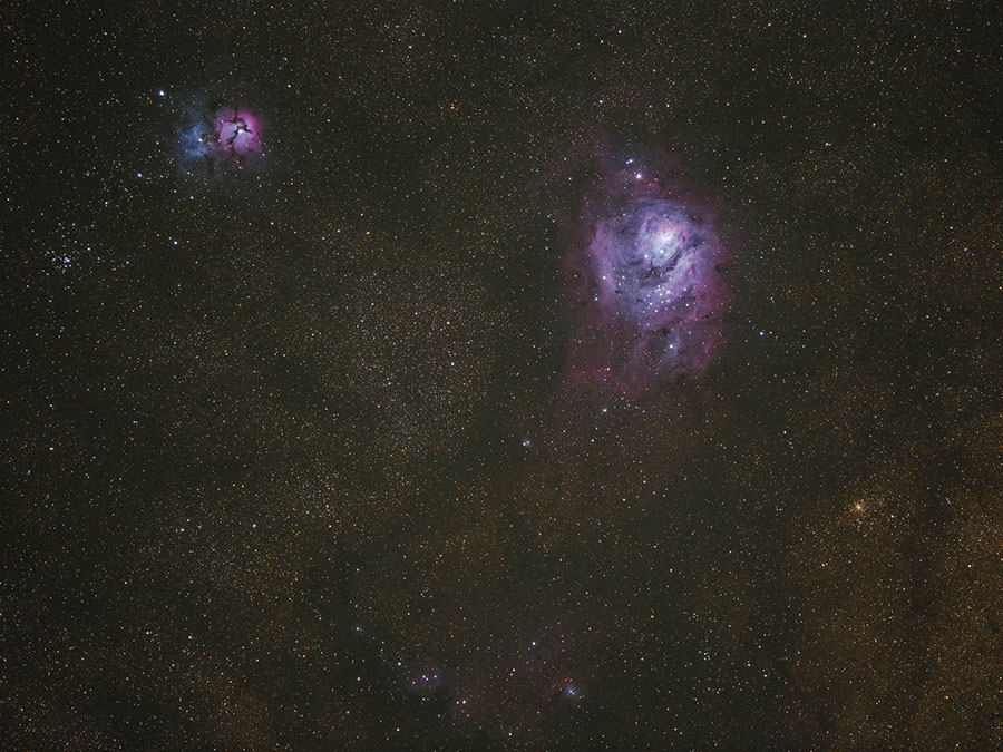
Single Exposure High Quality Dark Site Sub – 7 minutes @ ISO 400 – 5D III – f/4.5