Welcome to the PixInsights series. This series aims to provide a different kind of PixInsight tutorial. Rather than describe a start-to-finish canned workflow, the goal is to describe each tool in detail, and explain how they work. The ultimate goal is to give you understanding, rather than instructions, in the hope that will better equip you to use the tools PixInsight provides under any circumstances, rather than in a specific context. Please feel free to ask questions in the comments below. Discussion is key to learning.

BackgroundNeutralization

Like any image processing workflow, color correction is necessary to achieve properly balanced color in astrophotography. PixInsight supports a multi-step color balancing workflow, breaking up the process into a few key steps that allow the user to calibrate their images as they see fit using a number of different possible approaches. Foundational to all of these is BackgroundNeutralization (BN). This simple little tool is designed to balance out the color of your image background, which is an essential part of the color correction process. Neutralizing the background is itself not usually sufficient to produce properly calibrated color, although some may find that this process produces results they are quite pleased with and find subsequent calibration steps unnecessary. In most cases, BN will be followed up by a subsequent calibration step, such as PixInsight’s ColorCalibration or a G2V calibration routine, which will produce a fully calibrated image.

Basic Neutralization

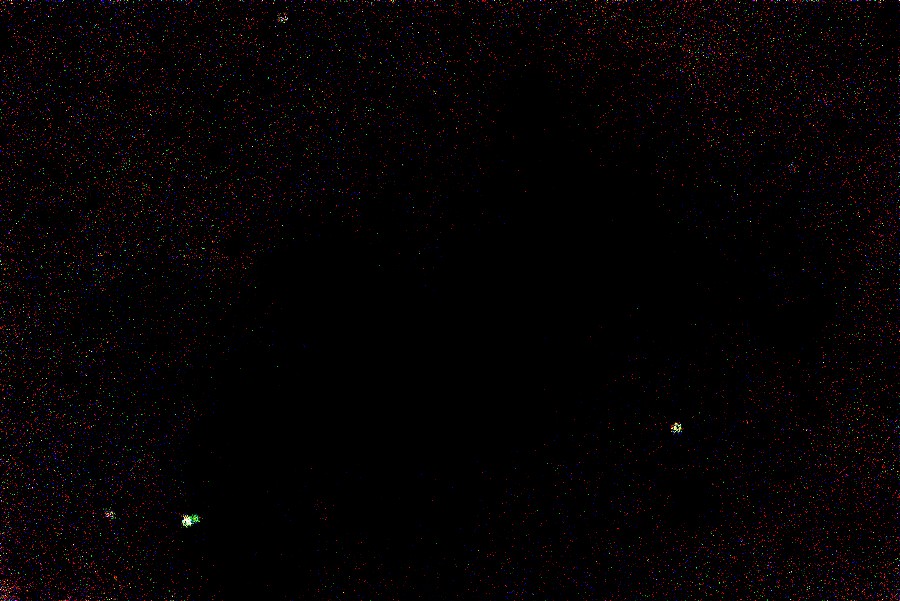
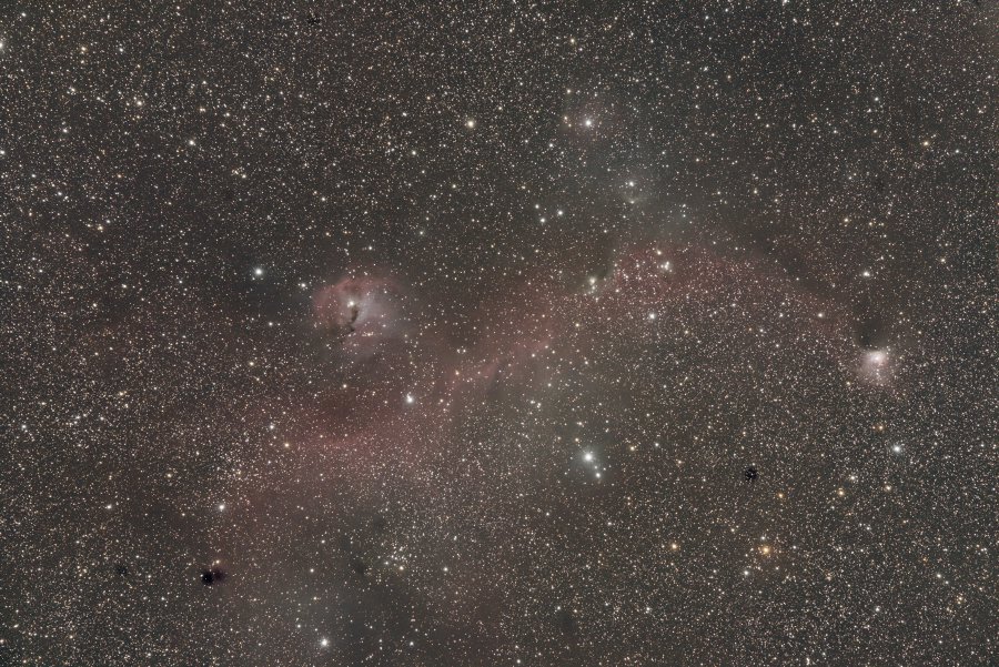
In it’s most basic use case, there is not a whole lot to using BackgroundNeutralization. Start by identifying a region of your image that represents the “true background sky level” with a preview. True background sky level must be chosen carefully here. You do not want to choose any region of sky that does not accurately represent the background sky. It cannot be a dust mote, a flare or reflection of any kind, and it should be devoid of any DSO content. You should avoid placing the preview in a vignette. If you still have vignetting at this point, then you should reconsider correcting that if at all possible, either by using flats when calibrating, and/or by using DynamicBackgroundExtraction. It can help to use the boosted STF option to get a better idea of where your darkest background sky is.

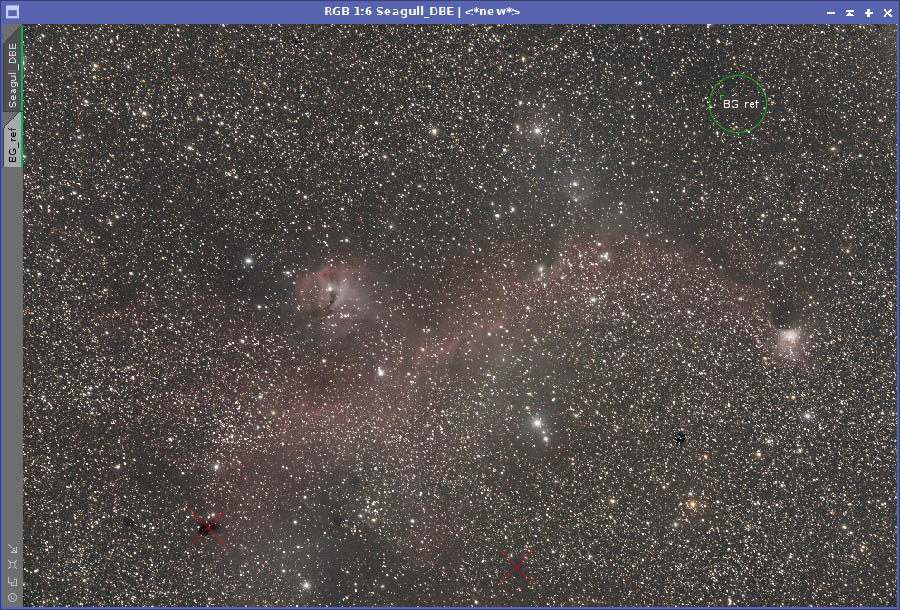
Choosing background reference (green circle); Avoid placing on dust motes (red xs)

When placing the preview, you should take care to avoid drawing the preview around any obvious stars. Stars in the preview can affect the accuracy of the background neutralization process, and should be avoided. Depending on the region of sky, you may be able to draw a larger preview, but in most cases, it will need to be fairly small. Galaxies are one subject that usually has a good deal of empty, truly neutral background sky, however most other images will either have some amount of nebula in them (even some galaxies if the field contains IFN) or too many stars to support a large preview.

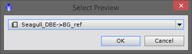Once you have your background preview, it’s best to rename it to “BG_ref” for easy identification. Open up BackgroundNeutralization, reset the tool, and choose your preview as the Reference Image. Leave all other settings at their defaults, and drag the triangle icon from the lower left corner of the BackgroundNeutralization window to your image to apply. By default, this will attempt to rescale the image data so it fits within the dynamic range without clipping. The image may appear strange immediately after application if this happens. In either case, once background neutralization has been applied, you will want to re-stretch the image using a linked STF. Since background neutralization is a part of color calibration, it is important that you apply STF with channels linked in order to see an accurate representation of what the process did to the color of your image. It also helps to make sure you have viewed the image with a linked stretch before applying BN as well, if you are interested in actually observing the difference.

For a basic neutralization, that’s all you need to do. You could continue from here and apply ColorCalibration or any other form of color and white point balancing that you prefer.

Configuring BackgroundNeutralization

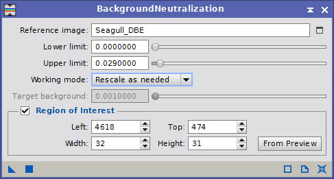
BackgroundNeutralization Tool Window

BackgroundNeutralization, while a fairly simple tool, does have a number of configurable options that you may need to use in certain circumstances. Most of these options you will never need to use, however one in particular I find quite useful. First off, let’s review the tool window options. The Reference Image is the image you wish to use as the source of your background reference. This may be either a preview in the image, as described above, or an entire image. Which of these you choose will depend on exactly how you are applying BN. The next two options are Lower limit and Upper limit. These two options restrict the range of pixel values or levels that will be factored into the calculations. These values set a range of exclusion, meaning the chosen value is inclusive in the excluded range. For lower limit, that means purely black pixels will never and can never be taken into account. For upper limit, it means all pixels brighter than or equal to your chosen value will be excluded. In most cases, you will never need to use lower limit. You may find that setting upper limit is useful, especially if you want the most accurate color correction, and particularly if you need to apply the same neutralization to many similar images (i.e. four panels of a mosaic where the background reference overlaps).

Working mode is one of the more important settings. Again, for most cases, you will never need to change this setting, which defaults to Rescale as needed. This option determines how BN will deal with scaling the data as a result of it’s neutralization of the background levels. The options are:

• Target Background
  • Will force the target image to have the specified mean level chosen in the Target background setting. This may result in some clipped data, however with this mode, only additive transformations are applied, so you may only clip on the high end (quite unlikely with most data, especially when using 32-bit or 64-bit floating point data). Image data from a CCD that had clipped stars, or image data from a DSLR at it’s base ISO that had clipped stars, may result in additional clipping with this mode.
• Rescale
  • Will always scale the pixels in the target image. Scaling is multiplicative, so no clipping will occur. This mode will force the image to utilize the full dynamic range, which may not be desirable depending on exactly how you intend to stretch.
• Rescale as needed
  • Will scale pixels in the target image only if required. Scaling is multiplicative as with Rescale, so no data clipping will occur. This is the default mode.
• Truncate
  • Will truncate pixels in the target image if they fall out of range (negative values or beyond the maximum value of the images working bit depth.) Special use cases.

Which working mode you use entirely depends on what you are doing and how you prefer to process your data. The default Rescale as needed will ensure that none of your original image data is lost. Depending on the kind of integrations you normally create, this may always result in rescaling, or it may very rarely result in rescaling. Images that are well separated from the left edge of the histogram, and have plenty of headroom before clipping whites, should never rescale.

Finally there is the Region of Interest. This allows you to specify a pixel coordinate for top/left and a width and height of the region of the Reference image you wish to use as the background reference. You can define this region manually, or you can generate it from a preview. This is useful if you need to neutralize many images that have the same field. This may be the case if you are working with several separate integrations that you will eventually be combining, or several copies of your image that you are processing differently, either for testing and comparison, or just for different aesthetic goals.

Advanced Usage

You may find that the default settings for BN do not serve your needs in every use case. Sometimes you may wish to force a certain background mean, or you may wish to avoid rescaling at all costs. If you are aware of the nature of your data, and are careful in your measurements, this is definitely possible. A couple of notes on the default behavior of BN. When you reset the tool, it will set upper limit to 0.1, working mode to Rescale as needed, and disable Region of Interest. For a carefully selected background reference where rescaling is not a problem, this is all fine.

Target Background Mode

When it comes to using alternative modes, namely the Target Background mode, understanding your data is very important. As this mode will scale the data additively, there is the risk that you could potentially clip star data. Whether that could happen depends on exactly what kind of data you loaded. PixInsight will load image data “unscaled” into a 16-bit integer space. For most linear CCD camera data, where gain is usually chosen to maximize the utilization of 16-bit data, very bright but unclipped stars could be close to the maximum value of 65535. Interestingly, because of the fact that PI loads image data unscaled, 14-bit, 12-bit and 10-bit DSLR or Mirrorless camera data will load in such a way that clipping is extremely unlikely to occur with linear data. The primary case where clipping may occur is if you choose a very high background value for target background, which will effectively add a very large offset to every pixel.

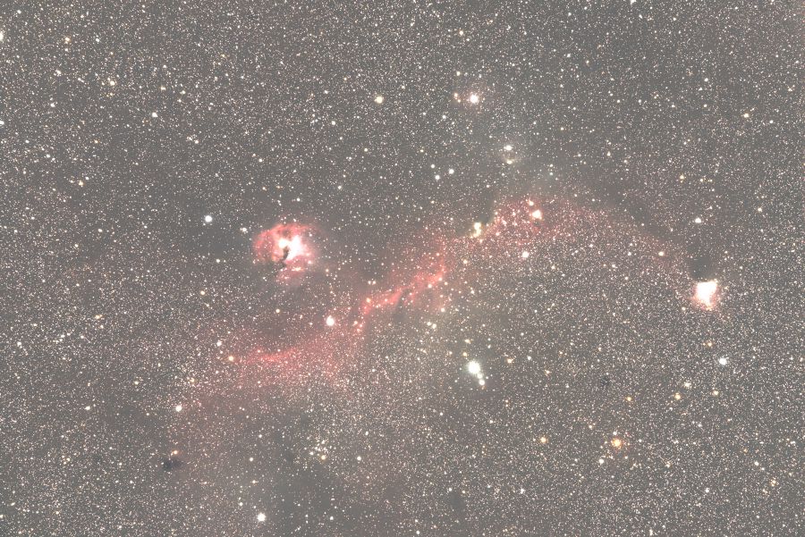
Target Background level 0.85

To demonstrate the kind of clipping that may occur when using Target Background mode, I’ve used a rather ridiculous value of 0.85 for the background level of the Seagull Nebula image originally used above to demonstrate background sky reference locations:
Using the pixel math formula iif($T == 1, 1, 0) on the image you can easily identify which pixels ended up clipping as a result if this neutralization:

Clipped Pixels from Target Background mode

In most cases, you will use Target Background mode in order to force a certain median background level. The most common use case would be to measure the pixels of your background reference preview. You can do this by selecting the preview tab, and configuring the pixel probe as demonstrated in this animation:

Set readout data to RGB/K, readout mode to Maximum, probe size to somewhere between 11 and 15, and normalized real range to 1E-05 or higher (depends on the precision of your data). Select the preview image and move the cursor around, and observe the readout (next to the black arrow you clicked to get the readout configuration menu). Set the background level to either the minimum or maximum of the values for the RGB channels. While you are measuring, make sure you exclude outliers. You can identify these by looking for pixels that appear to stand out in a particular way, such as the reddish pixel near the right center edge. Exclude these maximums from your evaluation of which level to choose for your background level:

In this case, the background levels range from ~0.0281 through ~0.0289, and either one of those would make for an acceptable level. I generally choose the larger, unless I have some other specific goal in mind, and apply BN to the image. Sometimes you may wish to force a specific background level. For example, if you know that you have a large separation in your signal, thoroughly separating the histogram peaks for each color channel from the left edge of the histogram, you may wish to choose a lower background level. Since Target Background mode operates additively, this can restore some headroom above clipped and/or bright stars in your image data (more useful with combined CCD RGB channels than with DSLR). Identifying the right level for this use case can take some trial and error, and using this simple pixel math expression, iif($T == 0, 1, 0), can help you narrow down the right background level with a few test attempts:

Clipped Background Pixels using low Target Background level

When the test image appears pure black, you are no longer clipping any pixels. If you check the histogram of such an image, you should notice the clipped pixel data riding up the right edge before background neutralization, and well-separated from the right edge after background neutralization:

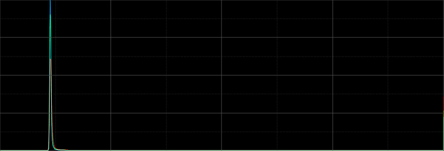
Histogram before BN with clipped pixels

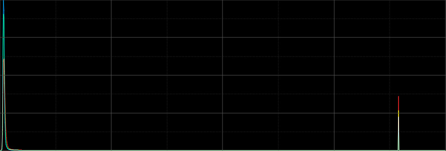
Histogram after BN with clipped pixels shifted well right

This is not a standard approach to removing an offset in your pixel data, however it is an effective one, and it kills two birds with one stone (without losing the linearity of the data, which is the particularly handy part.)

Rescale & Rescale as Needed Modes

More standard use cases for BackgroundNeutralization include the Rescale and Rescale as needed modes. Same as with Target Background mode, you will want to draw a preview around a region of true background sky. You will also want to measure the background level as demonstrated above, however in this case, you are specifically looking for the maximum level, across any of the color channels, while excluding marked outlier pixels (i.e. like the red pixel from the example above). This measured level should be set as the Upper Limit in BackgroundNeutralization to ensure the right range of background pixels is references for neutralization purposes.

Unlike Target Background mode, these two will rescale the data to make optimal unclipped usage of the available dynamic range. These modes will attempt to leave headroom and footroom in place above and below the extents of the signal. This tends to result in a total redistribution of information in the image, which requires that STF be reapplied to the image afterwards:

Rescale/Rescale as needed, before and after histograms

The image above exhibits a clipped signal, in many of the stars. Note the histogram before neutralization, where clipped pixels ride up the right edge of the histogram, and how they are separated from the right edge a bit after neutralization. Note that linearity is still not lost when using BackgroundNeutralization with a rescale mode, however the redistribution of tones does lay the foundation for proper color calibration, either with PixInsight’s built-in color calibration features, or with a third party option like eXcalibrator (G2V calibration).

Truncate Mode

The final mode of operation for BackgroundNeutralization is Truncate. This is a specialized mode that is not intended for normal background neutralization. To date, I have never found a specific use case for it, although PixInsight’s help tooltip indicates it may be used as part of intermediate processing steps. As I have not found any reasonable use for it yet, all I can do here is provide an example of what it does to the data, in comparison to the other modes. The following represent Target Background mode with a target level of 0.02, and Rescale/Rescale as needed with an Upper limit of 0.028:

Target Background (0.02)

Rescale/Rescale as Needed (0.028)

The following is an example of Truncate also using an Upper Limit of 0.028, as well as a pixel math test image that demonstrates the significant clipping that occurred as a result:

Truncate (0.028)

Truncated background pixels after BN

All three of these examples utilized the exact same background reference preview as originally defined in the section on basic neutralization. If nothing else, running BN in Truncate mode, then running this pixel math expression, iif($T == 0, 1, 0), on the resulting image, is a great way to identify dust motes in your image. The dust motes pop out quite readily as white or brighter areas of truncated pixels as in the Seagull Nebula example above (where I encountered several mobile dust motes, which moved around the frame every few shutter actuations).