PixInsights: DynamicBackgroundExtraction


Welcome to the PixInsights series. This series aims to provide a different kind of PixInsight tutorial. Rather than describe a start-to-finish canned workflow, the goal is to describe each tool in detail, and explain how they work. The ultimate goal is to give you understanding, rather than instructions, in the hope that will better equip you to use the tools PixInsight provides under any circumstances, rather than in a specific context. Please feel free to ask questions in the comments below. Discussion is key to learning.
DynamicBackgroundExtraction
 Background extraction is a key tool of the modern imagers software toolbox. As much as we may all desire to gather nothing but photons from deep space, that is rarely the reality of the hobby. Between light pollution from cities and the moon, as well as the low level ambient sky glow from Airglowand aurora, there is always an extra signal in our images. An unwanted signal that disrupts the proper and natural state of the sky as it should be.
DynamicBackgroundExtraction, often referred to as DBE, is one of the two primary tools PixInsight offers for identifying and removing these unwanted gradients in our images. The other tool is AutomaticBackgroundExctraction (ABE), which operates on some different principals, but is often an easier and more effective way of removing gradients from certain types of images. DBE is designed to give the user maximum flexibility in identifying any gradients that exist within the image by allowing direct user interaction with the image. This is where the dynamic part of the name comes from. DBE also provides a couple of different ways of removing different kinds of gradients, as not all are the same.
The Basics
Before we dive into the specific details of each of the panels of the DBE tool window, let’s cover the basics. Dynamic tools in PixInsight must first be attached to an image. After opening DBE, clicking in the image window you wish to extract a gradient from will associate the DBE instance with that image. The image should be a linear image (i.e. not yet stretched), and it helps to use a screen stretch so you can see the image and the gradients within. A four panel grid will appear in the image, and you will be able to start placing background reference samples. DBE requires a minimum of three samples to function, however you will usually find that many more samples than that are required to successfully identify gradients.
Placing a sample is as simple as clicking in the image. Once a sample is placed, it may later be selected, removed, or moved to a different location by dragging. Samples identify background level details, and should be placed on parts of the image that represent “true background sky”, even though the actual brightness level of those pixels may be relatively bright compared to how bright they actually should be.
The term “true background sky” is important here. Every DBE sample placed in the image will influence the generated gradient. If a sample covers pixels that represent part of the deep sky object you have imaged, such as nebula or galaxy structure, the colors and brightness level of those structures could be removed, partially or wholly, buy the background extraction process. As such, it is very important that samples only be placed on areas of the image that do indeed represent true background sky. In some images, such as isolated galaxies with shallower exposure, that may be fairly easy. In other images, such as deeply exposed galaxies that contain IFN structure within the background, large nebula covering the field, molecular clouds, or even regions of the Milky Way core that are packed with dense stars, identifying true background sky can be more difficult. It is these more complex images where using DBE, rather than ABE, becomes essential.
It is possible to generate samples in an image as well. DBE contains settings that allow automatic grid-based placement of samples possible, and these settings can be attenuated to configure what parts of the image are automatically identified as background sky, and which are assumed to be something else. Samples will only be placed in areas that are identified as background sky. This is not the same as using ABE, as algorithmically DBE operates differently, however for images with slight gradients with lower brightness levels, generating samples like this can be quite effective. Beware of using it on images with IFN, however, as those structures can be as faint or fainter than the gradient itself.
Once samples are properly placed in an image, DBE provides three modes of application: Generate gradient only, subtract the gradient out, or divide the gradient out. For most true gradients, you will likely be subtracting them, as they are unwanted signal and should be entirely eliminated. In the case of some gradients, those caused by vignetting or other shading of the sensor, you will want to divide them, in order to restore proper brightness levels to darker areas identified in the gradient. DBE can be useful in a pinch for fixing vignetting, however as a matter of course the best solution for that is to calibrate your original data with flat frames.
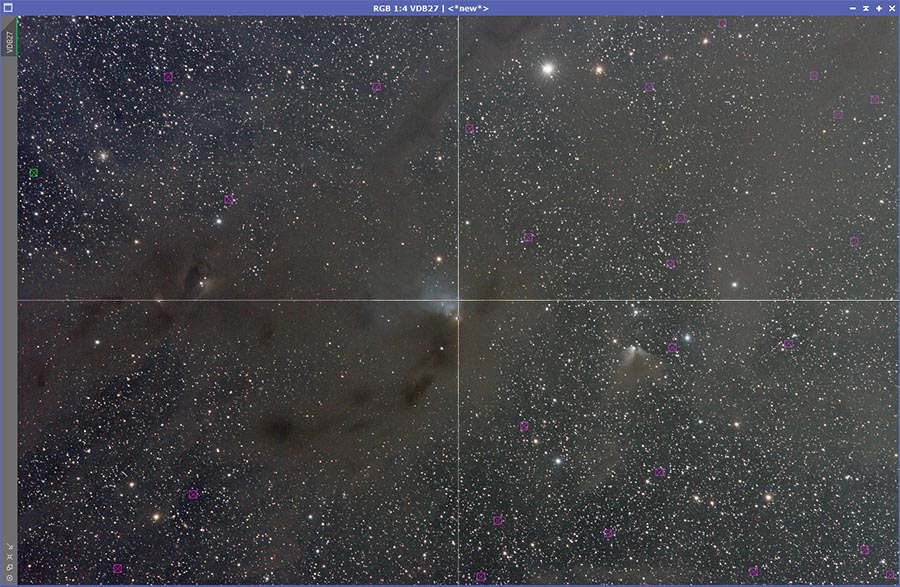
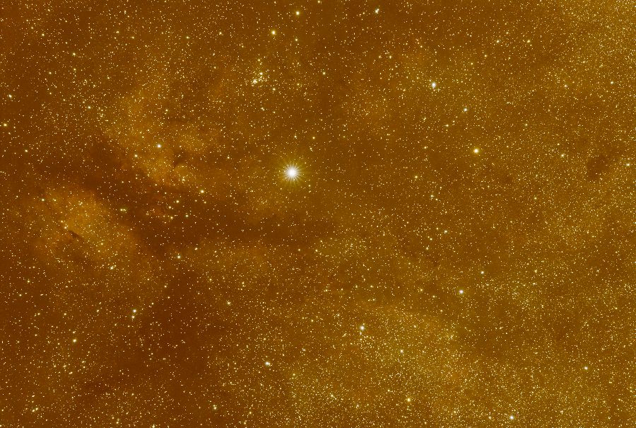
DBE Samples: Placed on true background sky in an image of dust and faint reflection nebula.
Gradient Identification

A proper gradient, extracted from the example image above
DBE may also be run without performing any action on the associated image. This will extract the gradient into a new image window and do nothing else. This is a very useful feature, and it should be used as a standard practice to check the identified gradient and determine which samples may need tweaking in order to identify the correct gradient. By correct gradient, I mean a gradient that has not inappropriately included any DSO colors. In some images, it may be fairly easy to identify when DSO colors have been included. Ha nebula or the golden color of stars near the milky way core will usually show up pretty well.
A proper gradient will usually match the color of the unwanted light. At a true dark site limited by, or mostly by, airglow, this will usually be a slightly brown color. At a moderate dark site that may be partially limited by airglow and partially limited by city light pollution, you may find that the LP is more silvery gray and the airglow takes on a more neutral color (still brownish, possibly tan). In the city, or with wider field images that dip into LP bubbles, you will likely find that gradients are decidedly more golden in color. Blues, magentas, reds are more likely to represent DSO content…nebula or galaxy structure. Note that these are simply general guidelines, and it is possible for much more complex gradients to exist within an image.
If imaging with a moon out, in just about any phase but a small crescent, you may find that your gradients take on a silvery sheen, however in some areas, where you may have a strong shift from airglow limited skies near one horizon (i.e. east), LP limited skies towards another horizon (i.e. south west), and the moon off towards a different horizon (i.e. west). In a situation like this, you may find that your gradient has blueish, greenish, even purplish colors in some areas (usually the corners).
Filters can also affect gradients. Narrow band filters should actually suppress them to a significant degree, with the possible exception of OIII closer to the moon on brightly moonlit nights. Color filters will often have different gradients from each other, depending on the potential light sources causing the gradients. Light pollution filters can result in very complex gradients. You may also find that blue and yellow corners show up opposite each other, and green and magenta corners show up opposite each other. You may find that the edges and corners are green, while the center is red, or vice versa. These kinds of gradients can be more difficult to extract, and will often require more meticulous tweaking of settings to identify the proper gradient and actually remove it.
In some cases, wild gradients may not actually be real. In some cases, quirks in the pre-processing steps, such as alignment or calibration and/or the stacking process itself, have introduced gradients. In most cases where this has happened to me with DSLR data, it has been a radial red/green gradient that was impossible to remove without redoing the pre-processing steps a different way. If you find that you simply cannot extract a gradient with DBE, this is usually the reason.
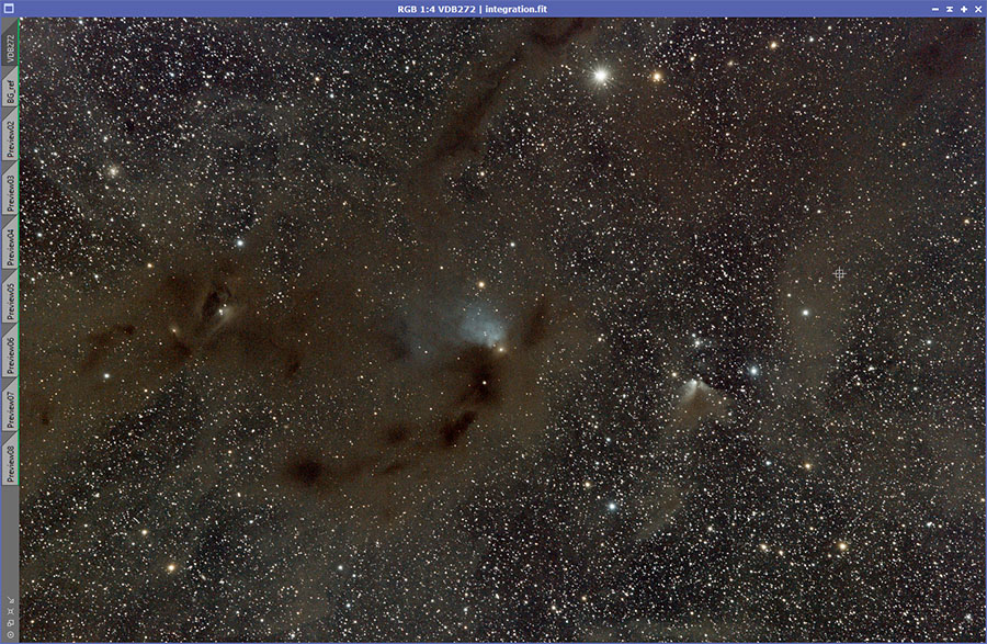
Image after gradient extraction with DBE
The Specifics
With the basics and general gradient identification out of the way, it’s time to get into the specifics of how DBE works. First off, there are several phases of working with DBE:
- Sampling
- Evaluation & Modeling
- Test Extractions
- Final Extraction
Before you can do anything with DBE, you must first place your samples. Once placed, you should evaluate the gradients identified, as described above, and tweak your samples to model the true gradient. Once you believe you have identified the correct gradient, you should test your extraction by NOT replacing the associated image. Finally, once you are sure your removing just the true gradient, you should do a final application to the associated image.
Before continuing, make sure your image is LINEAR and that you have applied a SCREEN STRETCH (unlinked, if necessary to eliminate color casts). DBE can be performed on stretched images, and there may be use cases that call for it, however for primary gradient extraction, it is best to apply it to linear data. Gradient extraction should be done EARLY in your processing. Gradients can affect color calibration tools like BackgroundNeutralization or ColorCalibration, and can skew the stretching process. Gradients represent UNWANTED SIGNAL, and it is best if that signal is removed promptly.
Sample Placement
Placing viable samples with DBE is the most important part of the process, and where you will spend most of your time. There are two possible approaches here:
- Automatic Sample Placement
- Manual Sample Placement
Depending on the contents of the image, you may wish to opt for one of the other. Images that have one or a few prominent objects separated by otherwise empty background sky will often work quite well with automatic sample placement. This includes galaxy images for galaxies away from the Milky Way, or images of small nebular objects that often have empty background space around them such as Wizard nebula or Pacman nebula. For most other images, a manual sample placement approach is usually ideal. Identifying true background can be difficult to impossible to achieve algorithmically, especially in the presence of complex or strong gradients (some gradients may leave a screen stretched image looking very dark in one corner, and very bright in the other, with the DSO “underneath” the gradient.)
Automatic Sample Placement
Automatic sample placement is a simple and quick way to get generally appropriate samples added to an image. To automatically place samples in an image, use the “Sample Generation” panel in the DBE tool window. You can start by simply clicking the “Generate” button. For square images, this will usually work like a charm. For images that are wider, you may wish to increase the count to 20 (for ~4/3 ratio images) or 25 (for ~3/2 ratio images). This will generate a tighter grid of samples that more fully covers the image.
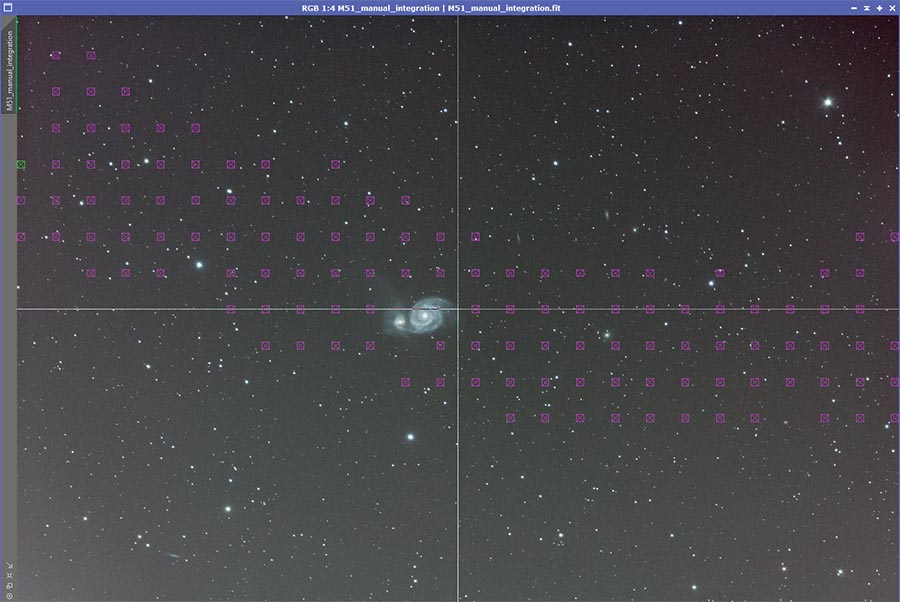
With the default settings, on an image that has no significant gradient, a moderate background signal level, and strong object signal, you should find that samples are placed on true background or faint object details, and nowhere on the object itself. In the case of a centered galaxy, for example, you should find that an even grid of samples is placed throughout the image except on the galaxy. This is “ideal” DBE behavior for placing samples, and is unlikely to be the case in most of the images you use it on, because if this was the case, you likely wouldn’t have any gradient to remove. A more typical image might be like this one of M51:
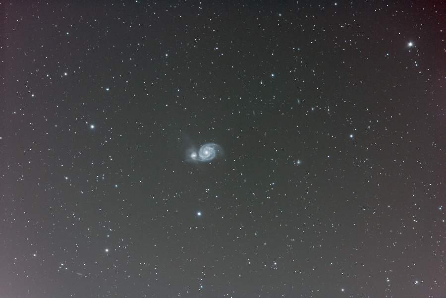
A galaxy image of M51 with a radial gradient (caused by a light pollution suppression filter.)
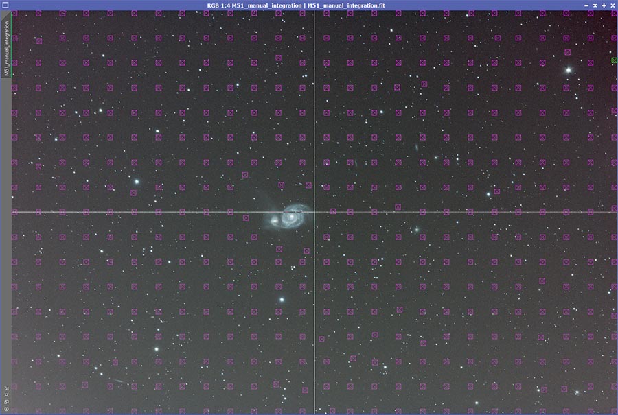
When you first generate samples on an image, you will likely find that the darkest and brightest parts of the gradient remain unsampled. You may also find they are distributed unevenly throughout the image. This is due to the default Modeling Parameters (1) settings. There are four settings in this panel that control the range of pixel brightness that can accept a sample. The Tolerance setting controls how bright the pixels can be, while Shadows relaxation controls how dark the pixels can be. With default settings (0.5 and 3.0 respectively), generating samples for the above image results in this sample distribution:
Initial sample placement with default DBE settings.
The samples fill a swath through the center of the image, from the upper left to near the lower right. Some of the fainter parts of M51 have been sampled as well. Interestingly, additional valid samples can be placed in some of the space between the existing samples, the dark upper right corner, and the bright lower left corner by clicking…however none are placed there automatically. This is due to the Minimum Sample Weight setting in the Sample Generation panel. It defaults to 0.75, which is a statistical weight of each sample’s brightness. To fill samples into the full range of bright and dark pixels allowed by the current Tolerance and Shadows relaxation, you can LOWER the Minimum Sample Weight. Reducing the min. sample weight will expand the range that samples can be placed, except (generally) in areas of the image that fall below darkness threshold set by shadows relax. or above the brightness threshold set by tolerance. It is sometimes possible that samples will fall into a “border” region along the darkness or brightness threshold…these will show up RED to indicate they will not be utilized for modelization purposes.
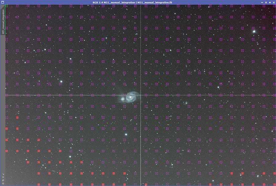
Gradient with min. sample weight of zero, with areas of the image still unsampled or ignored.
You may find that even reducing min. sample weight to zero, with the default tolerance of 0.5 and shadows relax. of 3.0, some parts of true background sky still do not end up getting sampled. This is the case in the above example. This is where we need to tweak either tolerance, shadows relax. or both. The kind of gradient in the M51 image here is a bit of a tough one, as that lower left corner and bottom edge are as bright as the DSO. In this particular image it won’t present as a big problem, however on some images, particularly those with very faint dust or very faint galaxy halo structure, having to expand the range of valid pixel brightness can result in samples being automatically placed on those actual structures. That can result in their partial or total extraction when the identified gradient is removed.
TIP: I have learned, through some of my struggles using a DSLR (relatively insentitive to light compared to a proper astrophotography CCD or CMOS camera), to trust my eyes when I feel I’m seeing faint background structure. Many more cases than not, when I have been left with faint fluctuations in background level that normally you would think were just blotch or some other kind of low frequency noise, investigations into deeper exposures of the same region revealed that the structures were indeed real. Faint, and often more blob shaped than filamentary as most space structures are, but real nevertheless. A proper first-pass gradient model will usually be quite smooth, and so long as it does not have localized color patches that will remove color from those faint structures, they will be left alone and in tact.
When you need to expand the range of samples when dropping min. sample weight to zero, it is best to increase it above zero, perhaps to 0.15. Here you want to switch to tweaking tolerance and shadow relax. to expand the allowed range of pixel brightness that samples can be placed on. In the case of our M51 image, samples have filled right into the darkest reaches of the image, but not into the brighter regions. That indicates we need to be more tolerant of brighter pixels, so we need to increase the tolerance setting in Modeling Parameters (1) panel. If the circumstances were reversed, we would want to relax the restrictions on darker (shadow) pixels (again with a larger number). It may even be that you need to adjust both settings to cover the full gradient. It is best to expand by a moderate amount, say +0.5 for tolerance or +1.0 for relaxation, then slowly pull the values back until you are no longer able to sample all the necessary parts of the gradient. Then push forward a little bit again.
With either setting, it is important to be moderate in your adjustments, and not overshoot by much. With tolerance, you have to be careful to avoid being so tolerant that you start sampling star signal. Generally speaking this is not a problem, however samples near brighter, bigger stars may start picking up star halo color, which could skew modelization. When relaxing shadows, it is similarly important to avoid supporting shadows so dark that you begin sampling field artifacts like dust motes or other unnaturally dark pixels. (DBE usually cannot fix those, as much as you may try, not at least without identifying object structure as well. Such artifacts are usually too small, although there are ways to model local gradient structure if you absolutely have to. There are better ways to model artificial flats that are usually more effective.) For M51, I ended up with a tolerance of 2.45 to get samples all the way into the corner.
When you have finally adjusted settings to place samples throughout all areas of true background sky, you are pretty much ready to go. There is one final step, however. If you had to relax the restrictions on modeling a lot, as was the case with the M51 image, you will usually need to examine the samples and remove any that fall onto any object structure. Simply select them by clicking on them, and hit delete on the keyboard. Alternatively, you can click the red X in the Selected Sample panel of DBE. This is a critical step in sample placement, as any part of your object or any structure that is sampled will factor into color calculations for that region of the modeled gradient. When the gradient is removed, it will either remove color from those areas, or screw with the color (depends on how you remove the gradient). In the case of fainter signals, which is usually the parts of object structure that ends up getting sampled by automatic placement, such as galaxy halo or faint nebula gas, this can completely decimate the color of those regions. So much so that those details may be lost into noise entirely.
Manual Sample Placement
Manual sample placement is necessary when you have complex image data to work with. This is especially true with images of large parts of or entire regional molecular clouds, regions packed with IFN, galaxies with large, faint extended halos, etc. Manually sampling an image uses the same settings and generally follows the same rules as automatic sampling. The key difference is that you are in total control over every sample placed. Manual sampling is usually necessary when you have an image so packed with content that you need very few sampled to properly identify the gradient without sacrificing true object structure. One of the more complex regions of space where this is often necessary is the extended molecular clouds within Cygnus, such as the huge regions of hydrogen and oxygen gas, infrared emission, and dust found around Sadr:
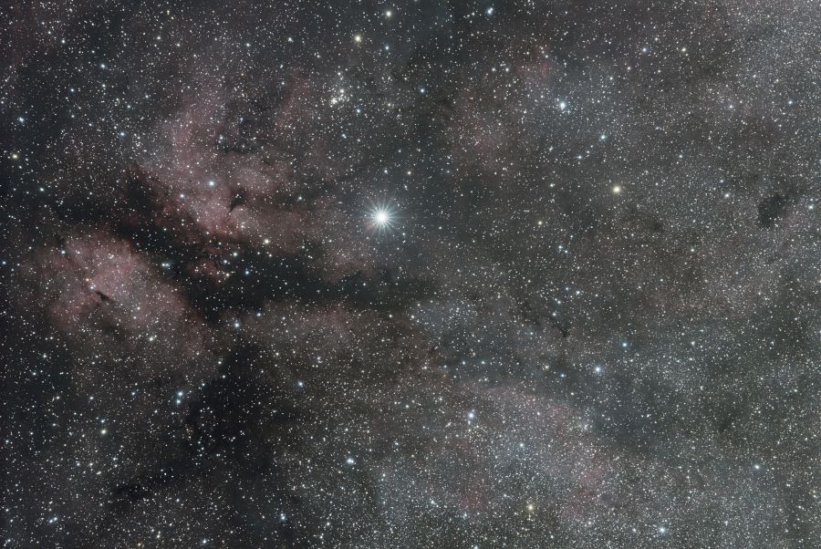
Sadr region of Cygnus, imaged with a DSLR with low Ha sensitivity leaving a complex field
This image demonstrates one of the most extreme examples of background extraction I have encountered in my own work. The image data was gathered with a camera that had relatively low Ha sensitivity (unmodded DSLR), allowing much more of the faint dust and what is most likely Oxygen nebula structure to show. There is also a definite gradient, brighter in the lower right and darker in the upper left. Manual identification of potential gradients is a key part of manually placing samples. They cannot be placed randomly, you must know where to they need to be placed. That requires identification of what is the likely primary gradient before hand. Not many images of space will have this much complexity in them, but these kinds of images are what DBE was made for.
Sadr region image with linked stretch
Before placing any samples, get a good feel for the gradient or gradients that exist within your image. It can be helpful to examine the image with both a linked and unlinked stretch, especially if the linked stretch has a heavy cast. The two may be quite different, and understanding the nature of a gradient in both modes will help you extract it properly. It also helps to know what is going on in areas of the image darkened by the darker parts of a gradient. Using a boosted stretch (usually unliked if you have an obvious color cast) can help you identify the nature of the gradient, nebula, and object structure in dark areas of the image.
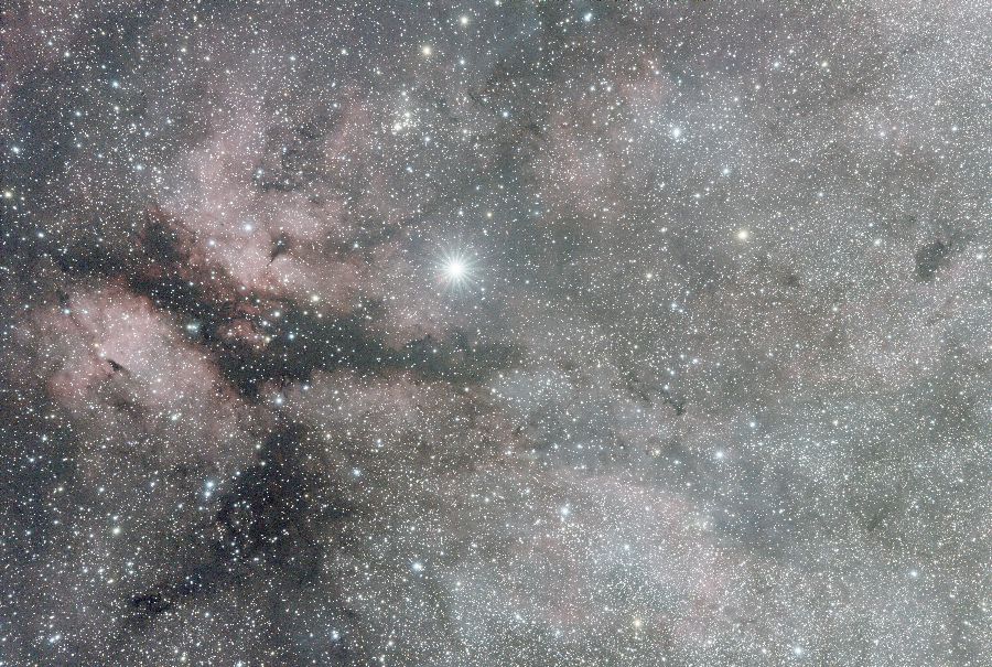
Sadr region image with unlinked boosted stretch
Based on the unlinked and boosted stretch images above, the likely gradient, which is not actually all that extreme but still present, is bright to the right/lower right and darkens to the left/upper left. This simple gradient is actually fairly easy to see in the unlinked stretch. The complex nature of the field, however, will limit any ability to extract that simple left to right gradient, so we will have to get as close as we can…without extracting any important nebula color. Preserving nebula color is by far the most important and difficult task with an extraction such as this.
To manually place samples in an image, you simply need to click once on the image to place. You can also click and hold, then drag to more precisely place a sample at a very specific spot, then let go. If a sample is placed incorrectly, you can click it to select, and drag to move. DBE maintains a list of all the samples placed in the image, and it is possible to cycle through them using the Selected Sample panel at the top of DBE. When a sample has been selected, you can cycle through them one at a time, in the order of placement, using the arrows in the Selected Sample panel.
Sample Tuning
SPARSE SAMPLE
After you have placed your sampled, either automatically or manually, you will want to evaluate them for accurate sampling quality. Not every sample will sample pixels well enough to identify and extract just the gradient. With big empty fields, which are common with galaxies, star clusters, and possibly some small, isolated nebula, most samples should be capable of sampling otherwise empty background sky, and will usually detect the proper gradient color. With more complex fields, getting your samples to detect the right colors can be a more complex task.
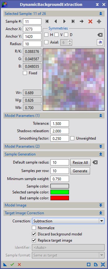
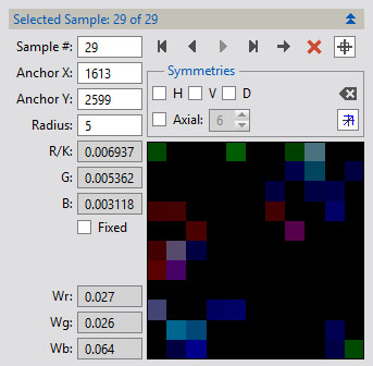
The Selected Sample panel is a very useful tool here, and offers some basic feedback that will help you evaluate whether a given sample is placed properly and sampling useful data or not. The big things to look for are whether your samples are picking up enough pixels, whether the pixels being picked up are providing useful information, and whether they are on stars. There are two low quality sample states that should be avoided: sparse samples and star samples. Neither are ideal, and both should be addressed as they could (although are not guaranteed to) lead to erroneous background modeling.
If a sample is too sparse (see SPARSE SAMPLE figure), much of the time DBE will automatically reject it, and it will appear red. Depending on your exact model parameters and minimum sample weight, some samples that are too sparsely sampling pixel information may end up being included and result in improper gradient modeling in that region. You can either relax your tolerances a bit, increase your minimum weight, move the sample, simply delete the sample, or possibly resort to more advanced sample tuning (see below).
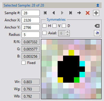
If a sample is on top of one or more stars (see STAR SAMPLE figure), you may be sampling bits of star halo data. That may not seem like an issue, however the outer regions of a star halo can be quite faint, and might possibly fall into the range of tolerance and shadow relaxation. Star halos are often quite different in color than the gradient you are trying to extract, and as such, should be avoided. Moving or deleting samples that fall onto stars is the best solution, although there may be some advanced sample tuning options (see below) that may allow a sample to remain viable in a star-crowded area.
STAR SAMPLE
A couple of other useful tricks with the Selected Sample panel can help you quickly move through samples in an image while you are tuning them. Near the middle top of the panel, you will find the sample cycling controls. You can jump to the first sample with the leftmost arrow, move to the previous with the second arrow, to the next with the third, and to the last with the fourth. This allows rapid movement through the samples currently placed on an image. If you have a lot of samples, such as may be the case with automatically generated samples, these tools may not be quite as useful. The fourth icon can often be quite useful, as clicking it will center a zoomed in view of an image on the currently selected sample. Finally, if you need to delete a sample, you can simply click the red X in the Selected Sample panel, rather than selecting the image viewport and pressing the delete key on the keyboard.
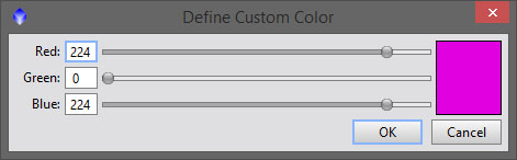
TIP: One more useful tip for sample tuning. The default sample color is gray, and in many images, that color can be very difficult to see. I will often change the default (unselected, valid) sample color to magenta, as that usually stands out quite well. Do this in the Sample Generation panel by clicking the Sample color swatch. Just drag the slider for the middle color (green) to zero, or simply edit the value to 0, and choose ok.
Gradient Evaluation
Evaluating the gradients identified by DBE’s modeling is arguably the most important part of performing a good background extraction.The nature of the identified gradient will affect the quality of the remaining data. A good extraction should, ideally, identify the gradient and only the gradient. DBE can be quite sensitive, and at it’s default settings, may often end up identifying and modeling aspects of your image that are not representative of gradient. This may result in a reduction in object signal or a loss of some kinds of signal (i.e. nebula). In images with lots of background sky, erroneous modelization of the gradient can usually be fixed just by shifting some samples around. In images as complex as my Sadr Region image used as an example above in manual sample placement, fixing erroneous modeling may require much more careful effort.
To evaluate the gradient modeled by DBE, set the Correction option in the Target Image Correction panel to None. Then apply to the image. This will model the gradient, and generate a new image window containing it. With linear images, you will need to stretch the gradient to see it. Continuing to use the Sadr region image as an example, I placed 26 sampled around the image where I thought they would best model the gradient I was seeing, and generated the gradient image. I stretched the image both with a linked stretch, and an unlinked stretch, to evaluate in both forms (these images are 50% their original size, so click to view at a larger scale):

Sadr – Linked Gradient – First Model

Sadr – Un-linked Gradient – First Model
The issues with this model should be fairly obvious. For one, it demonstrates pockets or “hot spots” of light and dark, rather than a consistent grade from one side/corner to another. In the unlinked stretch, you can also see faint pockets of color (sorry, JPEG compression muted those colors a bit, despite a very high quality setting). The bit of blue, red, and yellow-orange will be removed from the image if this model was used to remove the gradient. The low saturation of the color may seem trivial, however even a small amount of color such as this, removed via gradient subtraction, can reduce or eliminate color in your image. When dividing out the gradient, it can result in strange color shifts. Even a small amount of color removed from what may seem like a subtle amount of nebulosity can actually have a significant impact on your later ability to enhance that color (which, with other tools in PixInsight such as ColorSaturation, which lets you very selectively target and enhance narrow ranges of color). Note the reduced distribution of hydrogen nebula in the crop here after extracting the above gradient (click to see larger image):
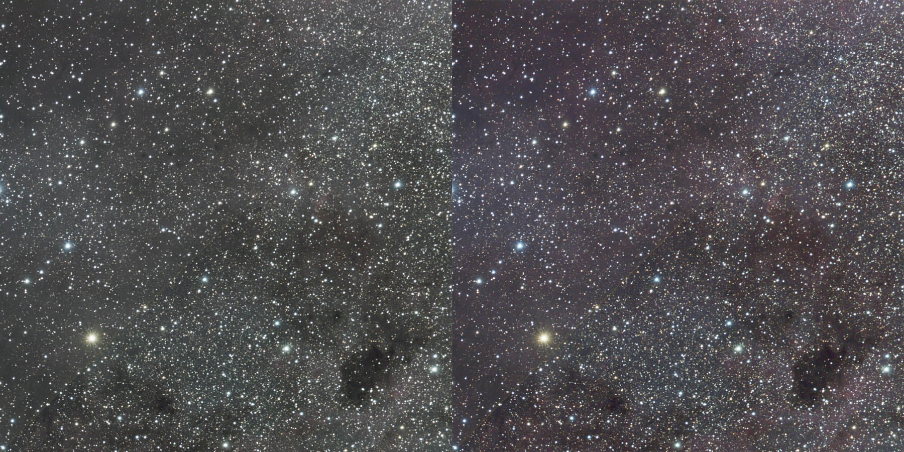
Sadr – Test Extraction – Loss of Ha
In the image above, the top triangle is before extraction, the bottom is after. Even with a slight amount of enhancement via just a global saturation, you should be able to see the area around the lower left corner where Ha color was lost. In this particular image, the gradient I can “see” through the details in the unlinked stretch appears to be brighter to the lower right and along the right, darker to the left. The gradient appears slightly color cast in green as you move to the lower right, and slightly cast in blue as you move to the upper left. I would say it should be otherwise “neutral” everywhere else. Structurally, I see Ha scattered throughout, including in the lower and upper right corners, about the mid-bottm region, middle right region, and significant amounts around the middle left to top. I don’t want to remove any of that. After redistributing samples around and tweaking tolerance and relaxation a bit, I had a model that was close, but demonstrated too many localized pockets of coloration and more hot spots, albeit coloration closer to what I expected:

Sadr – Decent gradient, not smooth enough
The solution to this problem was the Smoothing Factor setting of the Model Parameters (1) panel. The default smoothing factor of 0.250 is often good enough for most images, especially those with mostly empty background sky. In a complex image like the region around Sadr, a higher smoothing factor may be required to balance the weights of each sample, eliminate localized color pockets, mitigate hot spots, etc. Increasing smoothing factor to it’s maximum, 1.0, I ended up with the final gradient:

Sadr – Good gradient
With increased smoothing, the gradient is much more neutral, demonstrates fewer pockets of color, the colors are closer to what is expected and perhaps more importantly do not contain the reddish-pink of Ha or the yellow-orange of stars, the nature of the gradient matches what is apparent in the original image.
Testing Extraction
After you believe you have properly modeled your gradient, you need to test the extraction. While a model may look good, it may not actually do what you need. To test an extraction, change the Correction setting in Target Image Correction to Subtract. For most gradients, subtracting the gradient is the proper course of action. The gradient represents an unwanted signal, and thus it’s removal is desired. If you are using DBE to identify and remove a vignette
Testing the original modeled gradient before increasing the smoothing factor removed some nebulosity color, and left more of a green color cast, while not fully removing the gradient:
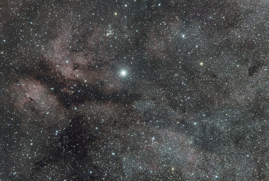
Sadr – First Test Extraction
The colors of the upper right in particular were lacking the Ha that was present in the original image. Increasing the smoothing factor and further tweaking a couple of points to reduce color casting in the gradient finally gave me the image I was looking for:
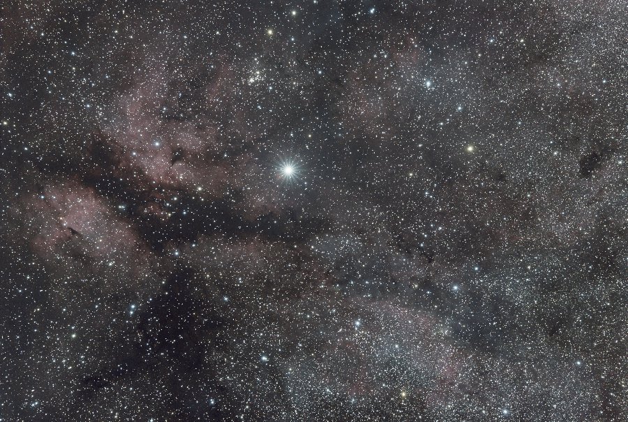
Sadr – Second Test Extraction
It is important to evaluate the subtleties of the test extractions, look for odd color casts, reduction or loss of important colors, etc. PixInsight is a powerful tool, and it has the capability to enhance even the most faint of faint signals, if they are not first lost through preliminary processing like DBE. The above tests were evaluated with an unlinked stretch. Remembering the color of the original image with a linked stretch from the manual sample placement section above, there was a very heavy orange cast to the image. It is also important to look at the image with a linked stretch, and examine the results. With the Sadr image, I chose to extract the background gradient without enabling the Normalization in the Target Image Correction panel, which resulted in the following color:

Sadr – Final linked gradient extraction
Normalization is a process that adds (when subtracting a gradient) or multiplies (when dividing a gradient) the final gradient-extracted image by the median value of the original image. This has the effect of preserving the original color balance of the image. Proper background extraction can have a fairly significant color-correcting behavior to it, as evident by the linked stretch test of the Sadr image above. Depending on your workflow, this may or may not be appropriate. With DSLR or OSC CCD images, the chances are that DBE is one of your very first steps, and usually performed before any other form of color calibration. In this case, extracting your gradient without normalization is probably most appropriate, as it will generally correct any color cast inherent in the linked stretch. In the case of monochrome CCD images that may be combined from separate color channels, it is fairly common to perform a linear fit across all the separated color channels before combining and performing colored background gradient extraction. Linear fit also has the effect of balancing color, and many imagers prefer the color balance that linear fit alone provides. In these cases, enabling normalization is necessary to preserve that original color balance.
Finally, when you are satisfied with your test extractions, simply enable the Replace target image option in the Target Image Correction panel, and click the green check mark at the bottom left of the DBE window. This will apply the gradient extraction to the image bound to DBE. Once gradient extraction is completed, remember to close the DBE window, as this is a dynamic tool.
NOTE: Regarding the color balancing effect that DBE may have when using it with Normalize disabled is unlikely to be accurate in any specific way. It can and usually will improve the color of images that exhibit strong color casts, however it is more a side-effect of the extraction process than anything. For ideal color balance, one should still perform a BackgroundNeutralization at the very least, possibly followed up by ColorCalibration or a G2V calibration procedure (such as with eXcalibrator).
As a final note, sometimes a single gradient extraction is insufficient for some images. There may be more complex gradients that cannot be modeled in a single pass, or you may be correcting a vignette as well as extracting a gradient. Performing multiple passes of DBE is a viable option, and sometimes necessary, especially with images that have a lot of open sky (galaxies and clusters) where smaller gradients are often very visible after the initial gradient extraction. When performing secondary extractions, you will often find that you need to loosen shadow relaxation even more, and may need to tighten up tolerance.
Advanced Topics
The DBE procedures described above cover the most common use cases for this tool. There are additional use cases, such as vignette correction and secondary extractions that I’ve noted before, that often require more advanced techniques to perform most effectively. Beyond the average use cases, DBE is a feature-rich tool that contains a lot of settings, not all of which are obvious in their meaning. In these advanced topics, I’ll cover each setting DBE has to offer in detail, and also explain how to perform some of the more advanced use cases. Before getting into more advanced gradient modeling and extraction procedures, I’ll cover the specifics of each section of the settings panels available in DBE, so you can apply those techniques to your images when performing standard or more advanced extractions. At this point, I am assuming that the settings in the Sample Generation panel are well enough understood, so I will not cover them in detail.
Model Image Tuning
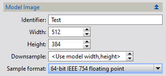 One of the key things DBE does is generate a gradient model image. This is the image that contains the gradient identified by the samples you have placed in your image, and modeled according to the settings you have chosen in the Model Parameters panels. For the most part, you should never need to change these settings, however sometimes you may find them useful if you wish to perform more advanced techniques such as manual extractions with pixel math.
The setting you will likely use most often is Identifier. By default, the model image will use a identifier derived from the image DBE is currently bound to, appended with _DBE. If there is already an image named <bound_image>_DBE, then a number will be added in sequentially increasing order: _DBE2, _DBE3, etc. One key reason to rename the model is if you intend to use it in some subsequent process, such as manually extracting the gradient with PixelMath.
In addition to identifier, you have the Downsample option. By default, DBE will generate the gradient image at half the scale, or 1/4 the number of pixels, as the bound image. Since the gradient is technically only modeling low frequency content, it need not utilize a large number of pixels, and reducing the size of the model image can help save on memory and improve the speed at which the model is generated. If you are working with a particularly large image, such as from a modern DSLR or high resolution CCD like a KAF-16803, where pixel counts extend into the several tens of millions, adjusting this to 3 will reduce the size even more (to 1/9th the number of pixels). You can adjust this as high as 16, which is not recommended for most images as you are likely to end up with erroneous removal if the resolution of the model image is too low, or reduce it to 1, which would use the same size as the bound image. You can also set this to <Use model width,height>, which will enable the Width and Height inputs where you can specify whatever dimensions for the gradient that you desire.
Finally, there is a Sample Format option. This allows you to choose the per-pixel data format, or bit depth and number format, for the gradient image. Normally you will want to keep this the same as the bound image, however if you intend to use the gradient for some subsequent process that requires a different format, you can change this here. As an example, if you intend to run PixelMath on the gradient in 64-bit float, you may wish to generate the model in 64-bit float up front.
Model Parameter Tuning
 The most commonly used settings in DBE are found in the Model Parameter panels. There are two panels, Model Parameters (1) and Model Parameters (2). The vast majority of the time you will use the settings in Model Parameters (1), as this contains the Tolerance, Shadow Relaxation and Smoothing Factor settings discussed in more detail above. I will not reiterate the usage of the settings in this panel further here, other than to state that the explicit ranges of each are as follows:
Tolerance: 0-10
Shadow Relaxation: 1-100
Smoothing Factor: 0.0 – 1.0
There is one additional setting in this panel: Unweighted. This is a true/false checkbox, and it simply enables unweighted sampling. Every sample is given a weight, in each channel of the image if it is a multi-channel image. Weights range from, 1.0 (100%) to 0 (0%). A weight of 1.0 means the sample will factor in the full value of each pixel it contains, while a value of 0.0 means it will effectively be ignored. Checking off the Unweighted checkbox means that every sample will assume a weight of 1.0. If you do this, you must be certain that every single pixel covered by a sample is indeed absolutely representative of true gradient. In some cases, this may be necessary in particularly difficult situations, however the vast majority of the time it is unnecessary.
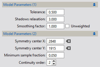
Additional settings can be found in Model Parameters (2). This panel contains the Symmetry Center, which I’ll go into more detail on in the section dedicated to symmetrical samples and background extractions. The other two settings are Minimum Sample Fraction and Continuity Order.
The first of these, Min. Sample Fraction, determines the minimum number of pixels that must be factored into a sample in order for it to be used. This value is a percentage, ranging from 1.0 (100%) to 0.0 (0%). It defaults to 0.05, which is 5%. The Tolerance and Shadow Relaxation settings of Model Parameters (1) ultimately determine whether a pixel is included in a sample or not. Those that are not show up pure black. In most cases, you will not need to adjust this setting.
Continuity Order is the final model parameter setting. This setting affects the accuracy of the model, however it also has the potential to introduce artifacts. For the most part, using an order of 2 (the default and also the lowest) is more than sufficient to accurately model a background gradient. If necessary, it can be increased up to fifth order. In testing, even orders, 2 and 4, produce accurate background models in most situations, and odd orders, 3 and 5, will usually produce inaccurate models. There may be specific circumstances with specific kinds of data where orders of three or five will produce a usable model, however to date I have not yet found such an image. I have also never needed to use a continuity order other than 2. It is best to leave this alone unless you have the mathematical knowledge to understand it’s potential benefits, and actually have a specific need to use it.
Advanced Sample Evaluation & Tuning
When it comes to samples, DBE provides the ability to accurately evaluate and very finely tune them. Most of this is done with the Selected Sample panel. This panel contains quite a few settings, some of which don’t have any direct impact on the sample’s contribution to gradient modeling, some of which allow you to control which sample you are working with, and some of which allow you to very finely tune the sample…which primarily means it’s level and color. I have already covered how to use the tools in this panel to move through the samples of an image, so I won’t go through those again. The main aspects of sample tuning that I will be covering here are the Radius, the color, the weights, the fixed flag, and how to use the sample preview to evaluate it’s contribution to gradient modelization.
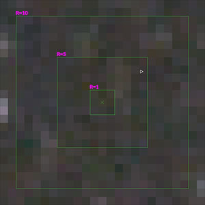
DBE Sample Radii: 10, 5 & 1
Before I go into tuning a sample, you need to understand the nature of a sample. Every sample in DBE is centered on a single pixel. The size of a sample, or it’s radius, is calculated not from that center pixel, but from the pixel next to it to the edge. The minimum radius of a sample is 1, however that means that the sample is three by three pixels in size, not one pixel in size. This is actually essential in order for a sample to actually be centered on a pixel, as otherwise samples with an even radius would never actually center on a single pixel. Thus, a sample with a radius of 5 is actually 11 pixels across, or represents a total of 121 pixels. A sample with a radius of 10 is actually 21 pixels across, and represents a total of 441 pixels. This should become apparent if you evaluate the number of pixels across in the sample preview, which is the large box in the Selected Sample panel that is usually filled with colored pixels.
An important note about sample radius. The radius of every sample can be independently customize by setting it explicitly in the Radius box in the Selected Sample panel. Setting the radius here will adjust the selected samples radius only, leaving other samples as-is. It is also important to note that changing the sample radius here will also change the default sample radius as well. This means that if you change the radius of one sample from 15 to 5, then add more samples by clicking elsewhere in the image viewport, those samples will have a radius of 5 rather than 15.
Every sample represents either a grayscale level, or a color value. This level or color value is specified in the R/K, G, and B boxes in the Selected Sample panel. These values are automatically chosen for you according to the sample weighting, which I’ll cover in a moment. It is possible to manually set the level or color of a pixel. This is done by enabling the Fixed option. When a sample is Fixed, it’s colors are automatically derived as the median of the colors from each channel…however you have the option of overriding those medians by filling out specific color values in the R/K, G, and B boxes if you so desire. Note that when working with linear floating point data, sample levels are usually very low, on the order of 0.001 or less. Extremely small changes in a sample value, on the order of 0.00001 or possibly even lower could have a very significant impact on a sample’s color or level. Generally speaking, you will never need to manually edit sample colors. If you have a problem with a sample, simply enabling the Fixed option is usually sufficient to overcome the issue.
The Sample Preview is your greatest friend when working a difficult gradient, such as the one in my Sadr region image from above. The sample preview shows you a representation of the weighted sample. By weighted, I mean how much of each pixel is being used to modelize the gradient. The weighting of a sample is directly related to the Tolerance and Shadows Relaxation settings. At their maximums of 10 for tolerance and 100 for relaxation, you might find that most samples have weights over 0.9, possibly over 0.99. To date, I have never found a sample with a full 1.0 weight…not, at least, without either using the Unweighted option in Model Parameters (1), or by marking a sample as Fixed. A Fixed sample is automatically weighted 1.0 in each channel.
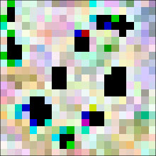
DBE Sample with Stars
The weight of a sample will affect the color of the pixels that show up in the sample preview. This is a very important aspect of sample evaluation. Comparing the pixels displayed in the sample preview to the pixels actually surrounded by the sample box in the image viewport will usually demonstrate fairly significant differences. The colors of a well-weighted sample will usually be similar to those of the actual image, however they will often have considerably different brightness, and some pixels may either be pure black, or may have aberrant colors.
The colors of the pixels in the sample preview are ultimately what affect the colors of the modeled gradients. When you have trouble modeling the proper color for a gradient, or trouble attaining proper neutrality of a gradient so it does not remove colors from your image that you do not want removed, tuning the colors of the sample pixels is the solution. In some cases, such as the Sadr region image, carefully tuning each and every sample to contain only a very specific range of pixel colors that precisely model the observable gradient is necessary. Reducing sample radius and carefully moving samples to contain pixels of just the right color range will improve modelization.
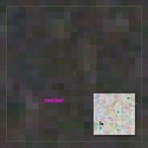
DBE Sample: Faint Star
To evaluate your samples, pay close attention to the colors within the sample preview. Pixels that show up black are pixels that have been under-weighted by the Tolerance and Relaxation settings of Model Parameters (1). If too many pixels show up black, according to the Min. Sample Fraction setting of Model Parameters (2) and the Minimum Sample Weight of Sample Generation, a sample will be ignored. The weighting can be adjusted by changing tolerance and relaxation, or simply by moving the sample around until its pixels fall within the accepted range set by the above mentioned settings. Sometimes just moving a sample is the appropriate course of action. Pixels that have aberrant colors are likely pixels that should be rejected, and are barely acceptable according to the restrictions set by model parameters. Most of the time, aberrant colors that do not neighbor black pixels are faint stars…generally too bright, but not bright enough to be entirely rejected. If your sample includes any stars, you will often find that bits of the star halo show up as aberrant colors instead of as black rejections. This is a key reason why avoiding stars in your samples is a good idea, as too many aberrant pixel colors can result in improper modelization.
Sample size also plays a role in what gradient color is detected. At a general level, larger samples tend to be better, as they tend to be more neutral, and small deviations in pixel color and level are averaged away as more pixels are included in a sample. For images with large regions of background sky, opting for larger samples that cover more pixels is likely better, as such samples will be less prone to influence from color casts introduced by background sky noise in one channel or another. On the flip side, smaller samples allow much more explicit sampling of very specific gradient colors. When it comes to images like the Sadr region image, smaller and smaller samples often become the saving grace of DBE, allowing more precision in identifying exactly the correct gradient. With greater specificity comes the need for greater smoothing, however…and you will often find that when you use smaller samples, you will also need to use higher Smoothing Factor values in Model Parameters (1), frequently the maximum of 1.0.
Secondary Extractions
Sometimes a single extraction is not enough to fully remove the gradients that may exist within your image. A single extraction may identify and remove a large scale gradient, only to reveal smaller scale gradients the original model did not identify or pick up. This is often the case when you increase the smoothing factor to intentionally reduce hot spots and color pockets that may otherwise damage your real image data. It may also be the case if your first extraction was to divide out a vignette, which I’ll go into more detail on in the Symmetry section below.
Secondary extractions tend to be more complex and often difficult than primary extractions. With a primary extraction your usually looking for a largely neutrally colored large scale grade across the entire image. With secondary extractions, you are often looking at pockets of unwanted color or more complex gradients that may not traverse the image in a consistent manner. With primary extractions, larger samples that more neutrally sample color information are usually ideal, however the same is often not true with secondary extractions. After one pass of gradient extraction color casts are usually more localized, so reducing the sample size with Default Sample Radius in the Sample Generation panel is usually warranted. I will often drop the size to 3, or even lower, to very narrowly target specific pockets of unwanted color. Click the Resize All button to update all the samples in the image.
…
Symmetry
DynamicBackgroundExtraction is a very powerful tool, so powerful in fact that it is capable of removing field vignetting when you are otherwise unable to take flats. Note that it will generally only remove vignetting, in most cases it won’t sufficiently remove dust motes unless they are of a larger scale and more diffuse. However when it comes to extracting a vignette, DBE can do a superb job. Extracting vignettes is a bit different than extracting gradients. Gradients are additional unwanted signal, and as such they are usually SUBTRACTED out of the image. Vignettes are different in that they are usually an unwanted loss of signal due to shading of the field by a part of the telescope, possibly a lens hood or scope dew shield, or some aspect of the imaging train. As they are a loss of signal, subtraction would only exacerbate the problem, so vignettes are usually DIVIDED out instead.
Identifying vignettes is often a challenging task with DBE in it’s normal mode of operation, with standard samples. Thankfully, DBE offers us symmetrical samples and field symmetry. Symmetry in DBE is a means of making assumptions about the structure of your field based on individual samples, or via axial structuring. Instead of placing multiple samples in each corner of your field, with symmetrical samples you simply enable symmetries for one or a very few samples placed strategically in specific corners of the image. A symmetrical sample will represent both it’s specified location, as well as it’s symmetrical locations. The color and weight of the symmetrical locations is based on the actual sample, rather than any actual pixels at the point of symmetry.
As vignettes tend to be symmetrical in nature, this allows us to very easily identify shading, usually in the corners of our image, and make the necessary assumptions that such shading will likely be consistent around the periphery of the field. With a perfectly collimated scope that has the sensor placed at the dead center of the optical axis, this “perfect” symmetry might actually be true. However in most cases, scope collimation is often not ideal, even if it may be acceptable, sensors may not be dead center of the optical axis, there may be tilt in the system, etc. These will all offset the center of the vignette from the center of the field.
To accomodate this, DBE allows the symmetry center to be adjusted. You already know of this feature, even if you did not know exactly what it was. When you first select an image to be used with DBE, you will notice that the image is divided up into four panels. These panels are created by two lines that cross the center of the image, both horizontally and vertically. The point at which they cross is the center of symmetry. These lines may be adjusted by pointing at them and dragging them around the field. You may also point at the junction of both and move the center wherever you please within the image viewport. By adjusting the center of symmetry, you can shift the points of symmetry of symmetrical samples, which will adjust the modelization of the vignette.
There are four types of symmetrical samples that DBE offers. Any sample can be turned into a symmetrical sample by enabling any of horizontal, vertical, or diagonal (HVD) symmetry. Any combination of these three symmetries may be enabled simultaneously, so a sample may have as many as three symmetries simultaneously. A fourth type of symmetry can also be enabled: axial symmetry. When axial symmetry is enabled, HVD symmetries are disabled. Axial symmetry allows multiple points of symmetry to be generated from a single sample, forming a polygon with anywhere from as few as three to as many as 24 vertices. Axial symmetries default to 6 vertices, and the general idea is to model the radial nature of the field around the optical axis (if the width and height of the image are the x and y axes, the optical axis is the z axis coming at you out of the screen). When standard symmetries do not work, axial symmetries might. Axial symmetries are also often the better choice for modeling LP bubbling in the center of a heavily vignetted field than standard HVD symmetries.
Finally, it should be noted that symmetrical samples can be mixed and matched with standard samples, and both HVD and axial symmetrical samples can be mixed and matched with each other. This allows very complex fields with complex vignetting and gradients to be modeled, often with very little effort.
Manual Extractions with PixelMath
(Section pending…)

Great Information on DBE and my images will surely benefit from improved implementation of DBE, but I would like to know what is “IFN?”
Jon, a very clear and helpful tutorial, especially as I’m currently working on a Cygnus widefield image with similar gradient challenges!
Wow Jon. This is great information on DBE. Apparently, I have been using DBE totally wrong. I really appreciate your insight provided within this tutorial. Thanks for you sharing this knowledge. I will begin using this information immediately.