Welcome to the PixInsights series. This series aims to provide a different kind of PixInsight tutorial. Rather than describe a start-to-finish canned workflow, the goal is to describe each tool in detail, and explain how they work. The ultimate goal is to give you understanding, rather than instructions, in the hope that will better equip you to use the tools PixInsight provides under any circumstances, rather than in a specific context. Please feel free to ask questions in the comments below. Discussion is key to learning.

LinearFit

The astrophotography data we image processors usually work with will most often come from cameras that have a non-linear response to different wavelengths of light. While a CCD or CMOS detector may be rated for some given quantum efficiency, say 56%, that is usually the peak response, and in the case of color detectors often the peak green response. The response of each pixel to other wavelengths, such as blue or red, or a narrow band channel like OIII, SII, Ha, etc. may differ. For the same exposure time, the resulting image intensity for each channel will often differ. This difference in image intensity across channels will usually result in some kind of color cast or even a strong color bias when the channels are combined. In the case of DSLR images or possibly OSC CCD, a strong color bias is usually intrinsic to the image.

In some cases, some imagers using monochrome cameras with external color filtration will often use inconsistent exposure times across each channel in an attempt to counteract the difference in response, gathering longer or shorter subs depending on which channel they are imaging in. This can improve color balance, but even with careful calculation one cannot account for the exact nature of a detector to any given range of wavelengths, so it is only a partial solution. For those using a sensor with some kind of color filter array like a bayer matrix, correcting non-uniform response at the time of imaging is generally impossible.

What is it?

Linear fitting is a process by which these differences in response to light are identified and corrected. Linear FIT might not be the most correct term to refer to the process used by PixInsight. According to one forum post on the PixInsight forums, a better description of the tool might be “Linear Matching”, as that is effectively what the tool does. PixInsight’s approach is to generate a set of pixel pairs from a reference image and a target image, and generate line from that set that represents the average difference between the two. The function that represents the line is then applied to the target image to match it to the reference image.

LinearFit could be thought of as a first-stage color correction tool. While it is not necessarily intended to give you accurate color calibration, it will give you data that is more consistent. This improved consistency allows you to process data that is likely to have more deterministic results, especially across processing attempts (as many of us like to do, as reprocessing old data with new skills is great way to breathe new life into old images.)

The Algorithm

A quick high level rundown on the algorithm PixInsight uses might be helpful for those who are interested in knowing exactly what this tool does. If one just went by the name, you might think that LinearFit generated a function for a line based just on the reference image, and applied that function to the target image. In actuality the algorithm is slightly different. Algorithmically, the procedure is as follows:

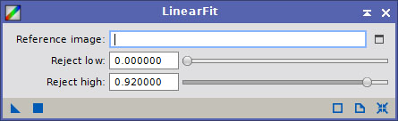
1. Generate set P from reference image R and target image T such that the following represents the set of all pixels within the two images that fall within the range defined by reject low and reject high:

   P := {{r1,t1}, {r2,r2}, ..., {rn,tn}}

2. Fit a strait line to all points in the set P, where r_i,t_i represents an X,Y coordinate in a plane.

   Y = mX + b

3. Apply the function that represents the line fitted in step two to all the pixels in T in order to match it to R.

The strait line fit in step two effectively represents the “average difference” between the pixels of the two images. This line is generated according to a variant of mean absolute deviation minimization. The slope (m) and y-intercept (b) of the fit line represent the deviation between the two images. If the target image is already fit to the reference image, the slope will be 1 and the intercept will be 0, resulting in no change to the target image. If there is any deviation, m will be greater or less than 1, and the intercept could vary quite widely (mostly due to noise and black point).

When to Use

Generally speaking, LinearFit should be used to normalize the color channels of your integrations before further processing is done, however it can have applications throughout the linear phase of an image processing workflow. For example, linear fitting integrations that are affected by strong background sky gradients will give you a more balanced linked screen stretch by may result in a skewed fit, and running a subsequent pass of LinearFit after primary gradients have been extracted can give you better initial color balance before any subsequent extractions are performed. LinearFit is best used as an initial step in your workflow, such that the benefits of working with deterministic data are gained as early as possible.

Data that has been linear fit and is deterministic becomes particularly important if you are combining narrow band channels, especially if you are combining with PixelMath. Without normalizing the intensities of your channels, determining the proper blends for each channel in PixelMath effectively becomes a guessing game, or you might need to perform additional steps in order to determine proper blending factors and offsets. Combinations performed without linear fitting the channels first will usually result in one channel totally dominatign, usually Ha as it tends to be the stronger channel, resulting in a strong color cast…red or green, depending on which channel you blend Ha into most.

A Narrow Band Example

With narrow band imaging, depending on any number of factors including different bandpasses, different amounts of LP, presence of the moon in the sky, the fact that Ha tends to be naturally more intense than SII or OIII in most cases, differences in sensor Q.E. for specific bands, etc. your channels may end up exposed to very different levels. When stretched with the same STF, using the darkest channel as a base, the offsets can be quite obvious. For example…a faint OIII, with a brighter Ha and even brighter SII:

When unaligned, unfit channels such as this are combined, the results can be a rather dramatic color cast, such as this orangish hue:

Narrow Band – UnFIT combination w/ color cast

By properly linear fitting the channels first, you can eliminate this color cast. Depending on the exact nature of your data, you may wish to fit SII, OIII and possibly NII to the Ha channel…however there can be benefits to fitting everything to the SII channel (notably, if you intend to do an SHO or “Hubble Palette” blend, as fitting to SII can help mitigate overpowering Ha). Once you have fit your channels, your combinations should begin to appear more reasonable:

Narrow Band – FIT Combination

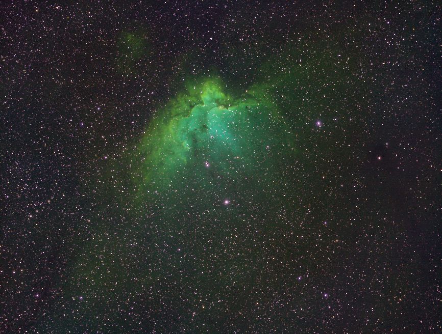
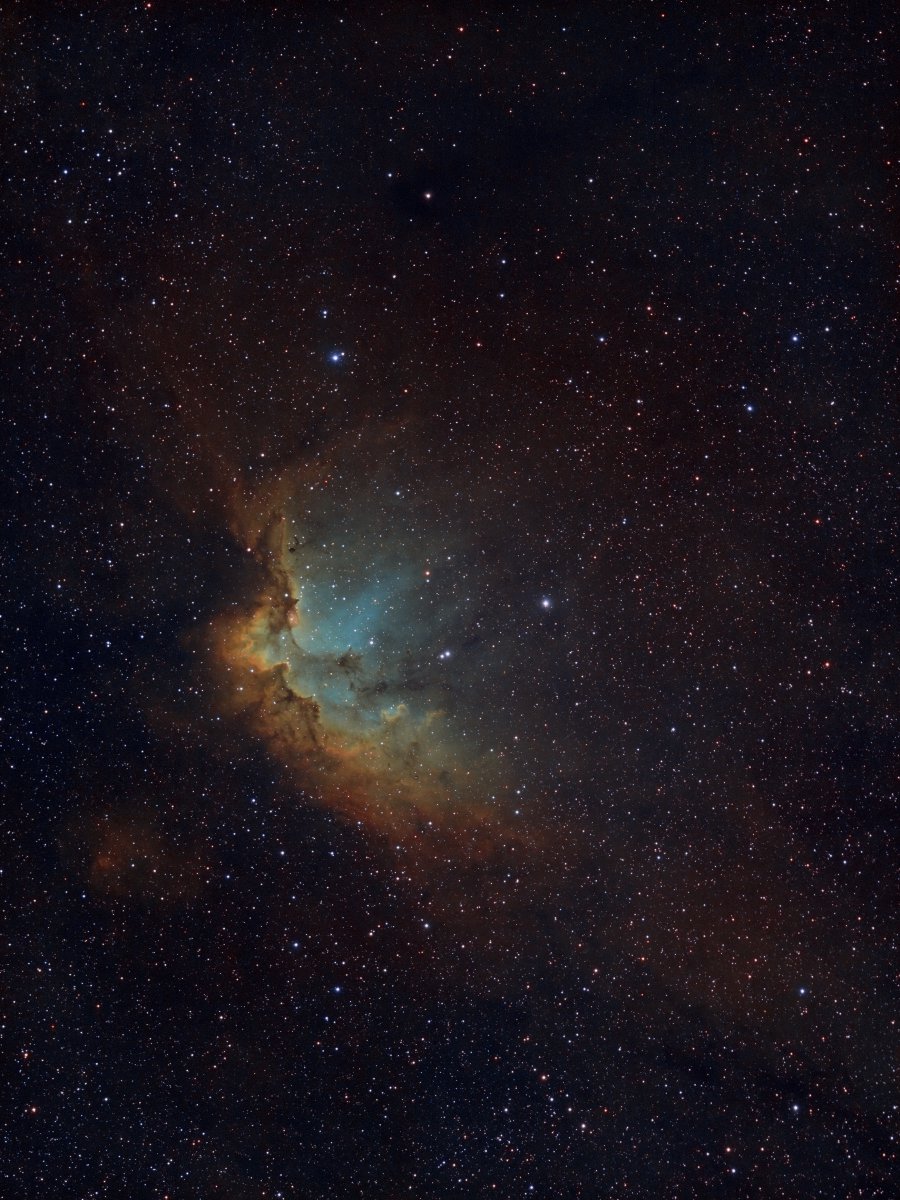
You may notice that your image still has a color cast in some areas, as in this example of Wizard nebula. This can occur when one channel, such as Ha here, is still much stronger than the others. Faint details are picked up in areas that are not yet picked up to a sufficient level in the other channels. This results in those channels being naturally weaker, allowing the dominant channel to exhibit most strongly in the color(s) it is combined into. The image here exhibits more green as Ha is most intense in most of these areas. The best solution to this kind of problem is to acquire more data in the weaker channels. However there are processing techniques that can be used, such as selective hue adjustments, that can produce a more balanced result (more on these in other articles):

A DSLR Example

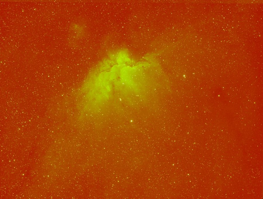
When imaging with a DSLR, and usually when imaging with an OSC CCD, very strong color casts, called color bias, can arise. These can be due to the presence of light pollution (often much more red in color than a true dark site background sky), airglow at a dark site (generally a faint brown), or the use of light pollution filters of some kind (IDAS LPS, Astronomik CLS, Orion SkyGlow, etc. which can range from reddish to heavily blue/green casts.) Here are a couple examples of this kind of color bias from images freshly integrated from DSLR RAW data without any additional processing:

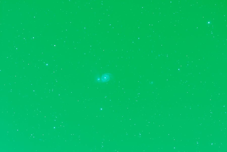
DSLR Color Cast – Green LP Filter

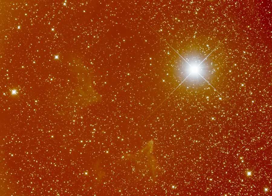
DSLR Color Cast – Orange LP

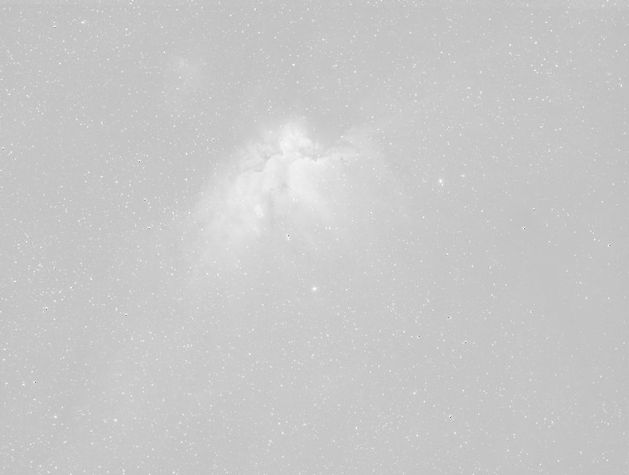
We’ll use the Ghost of Cassiopeia image here as an example of what linear fit does to an image. The orange color cast here is quite obvious, and is the result of heavy light pollution (despite the use of an IDAS LPS-P2 filter). The initial histogram (screen stretch) looks like so:

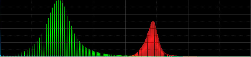
Non-fit Histogram

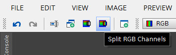To correct this initial color cast linear fit can be run on the split RGB color channels. To split the channels, you can either use the RGB mode of the ChannelExtraction tool and extract all three channels, or you could simply use the Split RGB Channels button on the main toolbar. Before actually splitting your channels, it is best to identify which channels has the lowest noise. This is best done with the NoiseEvaluation script, who’s output will be something like the following:

Calculating noise standard deviation...

* Channel #0
σR = 7.643e-005, N = 1050712 (6.26%), J = 4

* Channel #1
σG = 5.900e-005, N = 1804737 (10.75%), J = 4

* Channel #2
σB = 6.084e-005, N = 1891157 (11.26%), J = 4

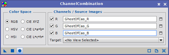
The channel with the lowest sigma (σ) has the lowest noise. That should be your reference channel, and the other two should be fit to it. To actually fit the target images to the reference image, you simply need to drag the small triangle icon in the lower left corner of the LinearFit window to the target image(s). After fitting is complete, you will want to recombine the separated channels back into a full color RGB image. This can be done with the ChannelCombination tool. Using the RGB Color Space, simply select the three separated channels you wish to combine, and hit the Global Apply button (the circle icon near the lower left of the ChannelCombination window).

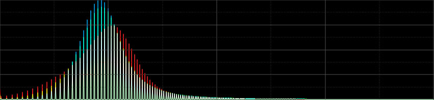
After recombination, you should be able to perform a linked stretch on the image, and see much more balanced color, devoid of any significant color cast (barring any that may come from gradients). In the case of the Ghost of Cassiopeia image from above, after fitting and recombining, the linked stretch looked like this:

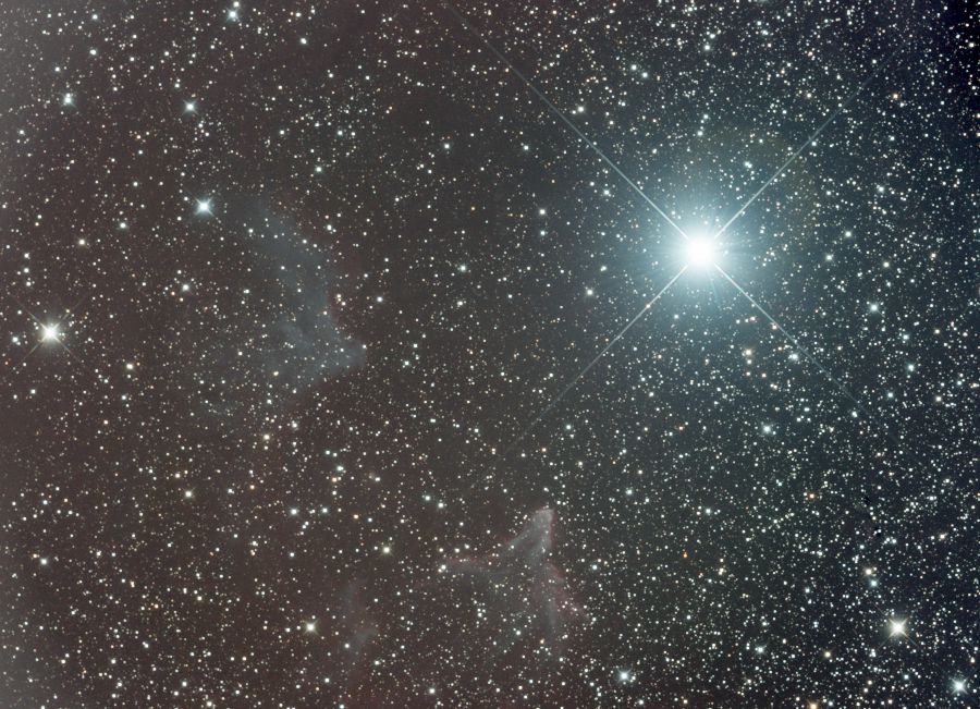
DSLR Linear Fit Result

The histogram of this fit image looks much better than the original:

When fitting your channels to the lowest-noise reference, you should find that the noise levels of the other two channels have dropped as well:

Calculating noise standard deviation...

* Channel #0
σR = 5.984e-005, N = 1050633 (6.26%), J = 4

* Channel #1
σG = 5.900e-005, N = 1804737 (10.75%), J = 4

* Channel #2
σB = 5.329e-005, N = 1891257 (11.26%), J = 4

The sigmas for each channel are now nearly identical, deviating by a fairly small amount relative to their original deviations. This should make it easier to maintain ideal behavior when running other tools on this data, including ABE/DBE, noise reduction, etc.

A Note about DynamicBackgroundExtraction

When linear fitting your image data, there is one thing to note about DynamicBackgroundExtraction. DBE has an option that supports working with data that has been LinearFit: Normalization. When the Normalize option is enabled in DBE, it will attempt to maintain the color balance of the original image. When Normalize is disabled, the process of extracting the gradient will generally have a moderate color balancing effect. If you have first fit your data, it is best to enable the Normalize option as that will preserve what LinearFit has done. Otherwise, it is best to leave Normalize disabled.